Abstract
In this chapter, we will illustrate the application of copulas in rainfall frequency analysis. This chapter is divided into two parts: (1) rainfall depth-duration frequency (DDF) analysis; and (2) multivariate rainfall frequency (i.e., four-dimensional) analysis. The rainfall data from the watersheds in the United States are collected and applied for analyses. The Archimedean, meta-elliptical, and vine copulas are applied to model the dependence among rainfall variables. Application shows that the DDF may be modeled by the Gumbel–Hougaard copula. Both vine and meta-elliptical copulas may be applied to model the spatial dependence of rainfall variables. Compared to the vine copula, modeling is easier to do when applying the meta-elliptical copula.
10.1 Introduction
Rainfall frequency analysis is of fundamental importance for hydrologic and hydraulic engineering design. In what follows, we will first introduce some examples with regard to rainfall analysis. Rainfall intensity-duration-frequency (IDF) or rainfall depth-duration frequency (DDF) curves published by National Oceanographic Atmospheric Administration (NOAA) are classic examples of rainfall frequency analysis. The IDF (or DDF) curves are derived first by separating rainfall events based on their durations (e.g., 15 minutes, 30 minutes, one hour, etc.) and then by fitting a univariate probability distribution to the rainfall depth or intensity data of a certain duration. The fitted univariate distribution is applied to produce a family of rainfall depth-frequency curves. In this manner, the two-dimensional depth-duration analysis is reduced to a one-dimensional analysis, involving only intensity (or depth) corresponding to a fixed duration. As described by the NOAA documents (e.g., TP-40), the IDF (or DDF) curves may be estimated from either annual maximum series or partial duration series. The IDF (or DDF) curves are widely applied in hydrological and hydraulic engineering design.
The rational method relates rainfall intensity (I) of a given duration (normally equal to the time of concentration) of a certain return period to peak runoff (discharge) (Q), where the peak runoff is assumed as a linear function of rainfall (Q = CIA)Q=CIA), where A is the area of the drainage basin. In this method, rainfall of a certain return period results in the runoff peak of exactly the same return period. To date, the rational method is commonly applied in urban hydrology (e.g., urban rainfall and runoff analysis) and urban hydraulic engineering design (e.g., detention/retention basin design, storm sewer design, and highway drainage design).
The SCS method, developed by Soil Conservation Service (now, the Natural Resources Conservation Service), may be applied to larger areas compared to the rational method (usually less than 60 acres [about 25 hectares]) for estimating runoff of a given rainfall amount. This method estimates the amount of surface runoff (or excess rainfall) through what is called the Curve Number (CN), which is related to land use and land cover, antecedent soil moisture, hydrologic condition, and soil moisture retention capacity.
The probable maximum precipitation (PMP) method, which does not rely on the IDF (DDF) curve, estimates the maximum amount of precipitation that may probably occur. The PMP analysis is required for the design of dams, dam breach analysis, spillway analysis, design of nuclear power plants, etc. These examples may be considered to illustrate applications of univariate rainfall analysis in hydrologic and hydraulic engineering design.
In the past three decades, bivariate (and multivariate) rainfall frequency analysis has attracted significant attention, because rainfall variables may be correlated and may significantly affect surface runoff (Cordova and Rodriguez-Iturbe, 1985). In the early days, the bivariate exponential distribution was applied to model the correlation structure of extreme rainfall variables (e.g., Hashino, 1985; Singh and Singh, 1991; Bacchi et al., 1994). Later, other bivariate rainfall models were investigated to model the relation between rainfall intensity and rainfall duration, for example, improved derived flood frequency distribution (DFFD) model by Kurothe et al. (1997) and Goel et al. (2000); Yue (2000a, 2000b, 2000c) investigated the applicability of bivariate normal, Gumbel logistic, and Gumbel mixed distributions. Besides the application to river discharge (Favre et al., 2004), the copula theory has been applied to bivariate and multivariate rainfall analysis (Grimaldi et al., 2005; Zhang and Singh, 2007a, 2007b, 2007c; Kao and Govindaraju, 2007, 2008; Cong and Brady, 2012; Zhang et al., 2012; Hao and Singh, 2013; Zhang et al., 2013; Abdul Rauf and Zeephongsekul, 2014; Cantet and Arnaud, 2014; Khedun et al., 2014; Moazami et al., 2014; Vernieuwe et al., 2015; among others).
With the advantages of the copula theory discussed in the preceding chapters, we will illustrate the application of copula theory to bivariate (or multivariate) rainfall frequency analysis. It is assumed that rainfall variables are continuous variates. However, rainfall variables may actually be discrete in nature.
10.2 Rainfall Depth-Duration Frequency (DDF) Analysis
Many studies have employed copulas for bivariate (multivariate) rainfall analysis based on annual maximum series (AMS). In this section, we will use Partial Duration Series (PDS) to illustrate the copula application to derive the DDF curves. The rainfall data with a 15-minute interval were collected for the rain gauge station: coop-166394 near Morgan City, Louisiana. The recorded data cover a period from May 8, 1971, to January 1, 2014. The rainfall data are available upon request from National Climate Data Center (NCDC).
The general procedure for DDF analysis includes the following steps:
1. Separate the rainfall records collected into independent rainfall events. Extract the rainfall depth and rainfall duration from these independent rainfall events obtained.
2. Evaluate the marginal rainfall depth and rainfall duration variables and corresponding marginal distributions.
3. Evaluate the rank-based correlation of rainfall depth and rainfall duration. Choose the possible copula candidates.
4. Perform the rainfall depth and rainfall duration analysis with the use of the possible copula candidates. Select the best-fitted copula functions.
5. Estimate the rainfall depth of given rainfall duration for a given return period.
In what follows, we will discuss how to perform the DDF analysis in detail.
10.2.1 Rainfall Data Processing
Before analyzing bivariate rainfall variables (i.e., rainfall depth and duration), we need to separate the rainfall data into individual rainfall events first. As commonly done, a six-hour duration of no rain is considered as the criterion to separate any two events. From a total of 12,089 available rainfall records for rain gage coop-166394, a total of 2,816 events were identified for the 43-year duration. Table 10.1 illustrates the rainfall event separation year 1971 as an example. From Table 10.1, it can be seen that there are nine independent rainfall events identified from May 22, 1971, to June 29, 1971. Table 10.2 lists the nine rainfall events separated. As an example, we consider the No. 5 event, which started on June 20, 1971, at 14:15 and ended on 15:15 on the same day. Summing up the incremental rainfall depths within this time window, we have the following:

Table 10.1. Illustration of rainfall event separation.
| Event no. | Date | Rainfall amount (mm)a | Interarrival time (h)b |
|---|---|---|---|
| 19710522 15:30 | 7.62 | — | |
| 19710601 00:15 | 0 | — | |
| 1 | 19710605 16:15 | 2.54 | 336.75 |
| 2 | 19710616 13:45 | 2.54 | 261.50 |
| 3 | 19710618 16:00 | 5.08 | 50.25 |
| 19710618 17:30 | 2.54 | 1.50 | |
| 4 | 19710619 13:30 | 2.54 | 20.00 |
| 19710619 13:45 | 2.54 | 0.25 | |
| 19710619 14:30 | 2.54 | 0.75 | |
| 5 | 19710620 14:30 | 2.54 | 24.00 |
| 19710620 14:45 | 2.54 | 0.25 | |
| 19710620 15:00 | 10.16 | 0.25 | |
| 19710620 15:15 | 7.62 | 0.25 | |
| 6 | 19710621 10:00 | 2.54 | 18.75 |
| 19710621 10:15 | 7.62 | 0.25 | |
| 7 | 19710622 20:00 | 12.7 | 33.75 |
| 19710622 20:15 | 5.08 | 0.25 | |
| 19710622 20:30 | 5.08 | 0.25 | |
| 19710622 20:45 | 5.08 | 0.25 | |
| 19710622 21:00 | 2.54 | 0.25 | |
| 19710622 21:15 | 2.54 | 0.25 | |
| 19710622 22:00 | 2.54 | 0.75 | |
| 19710622 22:30 | 2.54 | 0.50 | |
| 8 | 19710624 15:30 | 2.54 | 41.00 |
| 9 | 19710629 12:00 | 5.08 | 116.50 |
Notes:
a Incremental rainfall depth with 15-minute interval until the time stated.
b Difference between current day and time with the previous day and time.
Table 10.2. Nine rainfall events separated based on Table 10.1.
| No | Depth (mm) | Duration (h) | Max. Intensity (mm/h)a | Start | End |
|---|---|---|---|---|---|
| 1 | 2.54 | 0.25 | 10.16 | 6/5/71 16:00 | 6/5/71 16:15 |
| 2 | 2.54 | 0.25 | 10.16 | 6/16/71 13:30 | 6/16/71 13:45 |
| 3 | 7.62 | 1.75 | 20.32 | 6/18/71 15:45 | 6/18/71 17:30 |
| 4 | 7.62 | 1.25 | 10.16 | 6/19/71 13:15 | 6/19/71 14:30 |
| 5 | 22.86 | 1.00 | 40.64 | 6/20/71 14:15 | 6/20/71 15:15 |
| 6 | 10.16 | 0.50 | 30.48 | 6/21/71 9:45 | 6/21/71 10:15 |
| 7 | 38.1 | 2.75 | 50.8 | 6/22/71 19:45 | 6/22/71 22:30 |
| 8 | 2.54 | 0.25 | 10.16 | 6/24/71 15:14 | 6/24/71 15:30 |
| 9 | 5.08 | 0.25 | 20.32 | 6/29/71 11:45 | 6/29/71 12:00 |
Note: a Maximum average intensity of 15-minute interval.
Similarly, all rainfall events may be separated based on the six-hour duration of no rain criterion. Setting the threshold for the identified rainfall events as follows:
From the record, we have median = 7.62 mm and standard deviation = 23.87 mm, which yield the threshold = 31.49 mm. Applying this threshold, we reduced the number of rainfall events to 378 that is roughly about nine events per year. With the partial duration rainfall series thus identified, we can then start to investigate bivariate rainfall characteristics through (i) the investigation of the marginal distribution and (ii) the investigation of dependence.
10.2.2 Investigation of Marginal Distributions: Depth and Duration
Before we investigate marginal distributions, we will first look at a scatter plot of rainfall variables (Figure 10.1(a)). Zooming in on the lower-right corner (Figure 10.1(b)), we see there are ties in both rainfall depth and rainfall duration variables. The kernel density (nonparametric probability density estimation (Wand and Jones, 1995) is applied to approximate the nonparametric probability density and distribution function for univariate rainfall variables. The kernel density function is given as follows:
 (10.2)
In Equation (10.2), K(.)K. is the kernel function. Here we use the commonly applied K(x) = ϕ(x)Kx=ϕx, i.e., the normal kernel (the normal density function); h is the smoothing parameter, which is also called bandwidth (h = 6.086mm, 1.797hrh=6.086mm,1.797hr for rainfall depth and rainfall duration respectively); and n is the sample size.

Figure 10.1 Scatter plot for rainfall depth and rainfall duration: (a) original; (b) zoomed in at lower-right corner.
To compute the probability density and marginal probability using the kernel density, the MATLAB function is applied as follows:
In Equations (10.2a) and (10.2b), x and x1 represent the random variable and the data points where the nonparametric pdf and cdf need to be evaluated. Figure 10.2 plots the density function as well as the cumulative probabilities for both rainfall variables. The CDF estimated from the kernel density is applied for bivariate analysis using copulas.

Figure 10.2 Frequency and cumulative probability plots with kernel density function for rainfall depth and rainfall duration series.
10.2.3 Bivariate Rainfall Frequency Analysis
The scatter plot in Figure 10.1 indicates positive dependence between rainfall depth and rainfall duration. The rank-based Kendall correlation coefficient is computed as τn≈0.32τn≈0.32. Among the copula candidates (i.e., Gumbel–Hougaard, Clayton, Frank, Gaussian, and Student’s t copulas), the Frank copula is found to better model the bivariate rainfall characteristics. Figure 10.3 compares the empirical CDF estimated from the kernel density with the bivariate random variables simulated from the fitted Frank copula with its parameter value of 3.529. Comparison shows that (i) the simulated random variates cover the overall dependence fairly well; and (ii) the tie existing in both rainfall depth and rainfall duration variables may impact the concordance of the bivariate rainfall variables.

Figure 10.3 Comparison of bivariate empirical distribution using kernel density with the random variables simulated from the fitted Frank copula.
However, with the continuous assumption, we will proceed to estimate the rainfall depth for a given duration of a given return period. The exceedance probability (PexPex) corresponding to a given return period (T) for the partial duration series may be written as follows:
 (10.3)
In Equation (10.3), μ≈9μ≈9, the average number of events per year.
Equating Equation (10.3) to the exceedance probability of rainfall depth of a given rainfall duration, we have the following:
 (10.4)
Equation (10.4) is equivalent to the following:
 (10.5)
In Equation (10.5), CFrank(Fdep ≤ Fdep(x)| Fdur = Fdur(d)) = P(dep ≤ x| dur = d)CFrankFdep≤FdepxFdur=Fdurd=Pdep≤xdur=d. The conditional copula in Equation (10.5) is listed as #5 in Table 4.2. Applying the kernel density to the given durations of 1, 2, 3, 6, 12, and 24 fours, we have Fdur(d)Fdurd computed as follows:
For the return period of 1, 2, 5, 10, 25, 50, and 100 years, we have the exceedance probability computed using Equation (10.3) directly as follows:
Substituting Fdur(d), PexFdurd,Pex into Equation (10.5), we can compute Fdep(x)Fdepx numerically using the bisection method. Finally, we can estimate the corresponding rainfall depth using the inverse of the kernel density (fitted to the observed rainfall depth) with the computed Fdep(x)Fdepx. Table 10.3 lists the estimated Fdep(x)Fdepx and the corresponding estimated rainfall depth. Figure 10.4 compares the rainfall depth estimated from copula-based analysis with the published DDF of partial duration for Morgan City, Louisiana (http://hdsc.nws.noaa.gov/hdsc/pfds/pfds_map_cont.html?bkmrk=la). Comparison shows that (i) for the storms with shorter duration and return periods less than 10 years, the copula estimates are either closely following the NOAA estimates or well within NOAA 90% bounds; (ii) for short durations (i.e., D = 1 and 2 hours) and higher return periods (T ≥ 25 yr)T≥25yr), the copula estimates are higher than the NOAA upper 90% bounds; and (iii) as the storm duration increases, the copula estimates for higher return periods get closer to either NOAA upper 90% bounds or actually closely follow the NOAA estimates.
Table 10.3. Estimated probability distribution of rainfall depth and estimated rainfall depth of given duration with given return period.
| 1-yr | 2-yr | 5-yr | 10-yr | 25-yr | 50-yr | 100-yr | |
|---|---|---|---|---|---|---|---|
| Fdep(x)Fdepx | |||||||
| 1-hr | 0.5988 | 0.7364 | 0.8656 | 0.9252 | 0.9677 | 0.9834 | 0.9916 |
| 2-hr | 0.6512 | 0.7793 | 0.8921 | 0.9413 | 0.9751 | 0.9873 | 0.9936 |
| 3-hr | 0.7034 | 0.8195 | 0.9153 | 0.9548 | 0.9811 | 0.9904 | 0.9952 |
| 6-hr | 0.8296 | 0.9064 | 0.9599 | 0.9794 | 0.9916 | 0.9958 | 0.9979 |
| 12-hr | 0.9250 | 0.9622 | 0.9848 | 0.9924 | 0.9969 | 0.9985 | 0.9992 |
| 24-hr | 0.9594 | 0.9802 | 0.9922 | 0.9961 | 0.9984 | 0.9992 | 0.9996 |
| Rainfall depth (mm) | |||||||
| 1-hr | 55.30 | 68.64 | 92.78 | 116.32 | 166.01 | 206.38 | 246.33 |
| 2-hr | 59.54 | 74.73 | 101.12 | 128.39 | 182.26 | 221.99 | 261.82 |
| 3-hr | 64.72 | 81.89 | 110.86 | 143.97 | 198.76 | 238.62 | 277.24 |
| 6-hr | 84.01 | 106.74 | 151.78 | 193.73 | 246.69 | 284.32 | 314.98 |
| 12-hr | 116.25 | 155.60 | 211.31 | 251.90 | 299.25 | 327.08 | 350.48 |
| 24-hr | 150.98 | 195.86 | 250.48 | 287.99 | 326.54 | 350.01 | 370.53 |

Figure 10.4 Comparison of copula estimates with the NOAA estimations with a 90% confidence bound.
The differences between the NOAA-DDF and the copula-based DDF curves may be due to the following:
i. The NOAA-DDF analysis only extracts rainfall events for certain durations. These extracted events are then treated as univariate random variables and are fitted by univariate probability distributions.
ii. In the copula-based DDF analysis, on the other hand, rainfall events extracted may yield different rainfall durations. The bivariate rainfall depth-duration model is then constructed, and the rainfall depth of a given duration is estimated from the conditional probability function of f(depth < depth∗| duration = duration∗)fdepth<depth∗duration=duration∗. In this analysis, the duration can take on any value.
iii. The ties that may exist in the NOAA-DDF extracted events may not have the same degree of impact as that of copula-based DDF events. As discussed earlier, there may be many ties in the rainfall depth and duration of the extracted rainfall events (partial duration or annual maximum series), and these tied values may distort the concordance of the bivariate rainfall analysis. Additionally, the rainfall variables (especially rainfall duration) may be discrete in nature.
Even with the differences between the NOAA and copula-based DDF curves constructed for the partial duration time series, the copula-based method may be considered as a rational alternative for rainfall DDF (or IDF) construction with simpler and faster rainfall separation (events regardless of the length of rainfall duration) compared to that of NOAA analysis (rainfall duration–based directly).
10.3 Spatial Analysis of Annual Precipitation
With the assumption of annual precipitation amount as a random variable, the general procedure for spatial analysis of annual precipitation includes the following steps:
1. Select the region of interest, identify the rain gauges, and collect the annual precipitation records.
2. Evaluate the pairwise rank-based correlation coefficient of annual precipitation.
3. Identify the possible vine structure based on the rank-based correlation coefficients computed, and select possible copula candidates for T1 first, and then proceed with the analysis for the rest of the tree structure as discussed in Chapter 5.
4. Identify the proper tree structure for the asymmetric Archimedean copula and then proceed with the analysis as discussed in Chapter 5 for the asymmetric Archimedean copula.
5. Construct the meta-elliptical copula for the multivariate precipitation variables.
6. Compare the performance of different copula construction approaches.
To illustrate the spatial analysis of annual precipitation (rainfall), we will use four NOAA rainfall stations located in the Cuyahoga River Watershed, Ohio (see Table 10.4). The copula model is constructed from the annual rainfall data collected from 1953 to 2012 from NCDC. In this case study, we will apply D-vine, meta-elliptical copulas (i.e., meta-Gaussian and meta-Student T) and asymmetric Archimedean copulas. The reason that a D-vine copula is chosen from the pair copula construction is that there is no obvious center variable governing the dependence structure among all four rainfall stations (see the rank-based Kendall correlation coefficient listed in Table 10.5).
Table 10.4. Annual rainfall amount (mm) at four rain gauges.
| Year | Rain gauges | |||
|---|---|---|---|---|
| R330058 | R336949 | R333780 | R331458 | |
| 1953 | 668.528 | 634.746 | 536.702 | 744.728 |
| 1954 | 855.726 | 970.788 | 915.416 | 970.28 |
| 1955 | 705.866 | 943.61 | 943.864 | 872.998 |
| 1956 | 1,071.88 | 1,110.996 | 1,197.61 | 950.468 |
| 1957 | 735.584 | 954.532 | 859.79 | 839.47 |
| 1958 | 838.962 | 996.95 | 1,021.588 | 923.798 |
| 1959 | 1,025.906 | 1,334.008 | 1,240.282 | 1,075.182 |
| 1960 | 504.952 | 524.51 | 791.464 | 603.504 |
| 1961 | 716.026 | 773.43 | 909.828 | 930.656 |
| 1962 | 567.944 | 655.828 | 641.096 | 678.18 |
| 1963 | 437.134 | 535.94 | 499.11 | 503.428 |
| 1964 | 895.096 | 817.88 | 784.352 | 721.614 |
| 1965 | 754.38 | 757.682 | 912.876 | 757.682 |
| 1966 | 621.792 | 657.352 | 787.654 | 745.236 |
| 1967 | 676.656 | 684.784 | 822.452 | 917.194 |
| 1968 | 796.544 | 852.932 | 1,136.142 | 817.372 |
| 1969 | 738.632 | 786.384 | 1,152.652 | 768.604 |
| 1970 | 879.348 | 929.132 | 926.338 | 754.634 |
| 1971 | 684.022 | 826.77 | 786.638 | 628.142 |
| 1972 | 1,003.554 | 937.514 | 1,070.864 | 934.72 |
| 1973 | 841.248 | 940.054 | 1,013.714 | 1041.146 |
| 1974 | 899.922 | 1,041.146 | 1,021.588 | 1048.004 |
| 1975 | 933.196 | 1,049.782 | 998.474 | 1032.764 |
| 1976 | 759.714 | 892.556 | 767.588 | 1045.21 |
| 1977 | 54.864 | 957.072 | 1,027.684 | 1169.924 |
| 1978 | 699.262 | 829.31 | 910.336 | 805.434 |
| 1979 | 876.046 | 1,065.53 | 1,082.294 | 1132.586 |
| 1980 | 854.71 | 875.538 | 863.092 | 848.106 |
| 1981 | 881.38 | 914.4 | 970.534 | 897.89 |
| 1982 | 733.806 | 881.38 | 833.12 | 845.058 |
| 1983 | 885.19 | 984.504 | 1,007.11 | 851.916 |
| 1984 | 753.364 | 833.12 | 827.532 | 1026.922 |
| 1985 | 852.424 | 939.8 | 923.29 | 1,005.586 |
| 1986 | 721.106 | 850.646 | 934.466 | 1,125.474 |
| 1987 | 618.744 | 670.56 | 807.212 | 897.382 |
| 1988 | 735.33 | 721.614 | 744.728 | 773.938 |
| 1989 | 884.428 | 897.128 | 811.022 | 993.14 |
| 1990 | 1,592.834 | 1,193.546 | 1,251.712 | 1,347.216 |
| 1991 | 530.86 | 628.142 | 680.212 | 716.28 |
| 1992 | 1,019.048 | 1,010.412 | 1,069.34 | 1,020.064 |
| 1993 | 898.652 | 915.416 | 811.276 | 805.434 |
| 1994 | 909.066 | 867.41 | 852.17 | 788.924 |
| 1995 | 813.308 | 918.718 | 799.592 | 830.072 |
| 1996 | 1,128.014 | 1,097.28 | 979.424 | 1,168.146 |
| 1997 | 797.56 | 861.822 | 875.284 | 968.248 |
| 1998 | 978.662 | 970.788 | 869.442 | 963.168 |
| 1999 | 751.586 | 806.45 | 791.972 | 987.044 |
| 2000 | 1,013.968 | 932.434 | 969.518 | 887.222 |
| 2001 | 764.54 | 771.906 | 778.256 | 774.192 |
| 2002 | 931.926 | 744.982 | 891.54 | 837.946 |
| 2003 | 1,149.604 | 1,142.492 | 1,205.484 | 1,036.828 |
| 2004 | 1,049.274 | 1,088.136 | 1,056.386 | 956.818 |
| 2005 | 897.382 | 982.726 | 908.812 | 910.59 |
| 2006 | 1,053.084 | 1,087.882 | 1,160.78 | 1,362.964 |
| 2007 | 918.21 | 970.534 | 985.266 | 1,145.794 |
| 2008 | 887.984 | 1,012.19 | 963.422 | 1,165.606 |
| 2009 | 781.558 | 899.668 | 941.832 | 965.708 |
| 2010 | 774.446 | 846.328 | 747.776 | 927.862 |
| 2011 | 1,360.678 | 406.908 | 1,551.432 | 315.722 |
| 2012 | 782.574 | 664.718 | 849.122 | 782.828 |
10.3.1 Application of D-Vine Copula to Four-Dimensional Rainfall Variables
Copula Identification for T1
According to Kendall’s tau correlation coefficient matrix, the proper structure for T1 is as follows: R330058 − R333780 − R336949 − R331458R330058−R333780−R336949−R331458 (i.e., the bivariate pairs for T1 are [R330058, R333780]; [R333780, R336949]; [R336949, R331458]). Using the empirical marginals (Weibull plotting position formula), let U1, U2, U3, U4U1,U2,U3,U4 represent the empirical marginals as follows:

The D-vine structure for this example is the same as in Figure 10.5. In this case study, we choose Archimedean copulas for dealing with the positive dependence (Gumbel–Hougaard, Clayton, Frank, Joe, and BB1 copulas) as the candidates. Chapter 4 listed the one-parameter Archimedean copulas candidates. Hence we only give the formula for BB1 copula, which is a two-parameter Archimedean copula with the limiting conditions of either the Clayton or Gumbel–Hougaard copula. The BB1 copula (Joe, 1997) can be formulated as follows:
 (10.6)
The BB1 copula converges to (i) the Gumbel–Hougaard copula if θ1→0θ1→0; and (ii) the Clayton copula if θ2 = 1θ2=1.

Figure 10.5 D-vine structure for four-dimensional rainfall variables: (1) R330058, (2) R336949, (3) R333780, and (4) R331458.
In addition, the BB1 copula has both upper- and lower-tail dependence coefficients, as follows:

The parameters of T1 are estimated with the pseudo-MLE through the empirical marginals for all the copula candidates (Table 10.5). Table 10.6 also lists the log-likelihood, AIC, and BIC values with the best-fitted copula highlighted. From Table 10.6, we see that the two-parameter BB1 copula is the best-fitted copula for stations (R330058, R333780, R333780, and R336949), and the Gumbel–Hougaard copula is the best-fitted copula for stations R336949 and R331458.
Table 10.6 Estimation results for copula candidates.
| Variables | Copulas | θθ | LL | AIC | BIC |
|---|---|---|---|---|---|
| Gumbel-Hougaard (GH) | 2.7782 | 35.0603 | −68.1206 | −66.0601 | |
| Clayton (C) | 2.9226 | 33.9990 | −65.9979 | −63.9375 | |
| U1 v. s. U2U1v.s.U2 | Frank (F) | 8.8627 | 31.7661 | −61.5322 | −59.4718 |
| Joe (J) | 3.3021 | 28.8828 | −55.7655 | −53.7051 | |
| BB1 | [1.0203, 1.9788] | 39.0411 | −74.0821 | −69.9612 | |
| Gumbel-Hougaard (GH) | 2.3336 | 26.0645 | −50.1290 | −48.0685 | |
| Clayton (C) | 1.8549 | 20.2556 | −38.5113 | −36.4508 | |
| U2 v. s. U3U2v.s.U3. | Frank (F) | 6.8861 | 22.8811 | −43.7622 | −41.7017 |
| Joe (J) | 2.8627 | 23.0147 | −44.0294 | −41.9689 | |
| BB1 | [0.3841,2.0196] | 26.7981 | −49.5963 | −45.4754 | |
| Gumbel-Hougaard (GH) | 1.7527 | 22.9526 | −43.9052 | −41.8447 | |
| Clayton (C) | 1.2274 | 12.7401 | −23.4801 | −21.4197 | |
| U3 v. s. U4U3v.s.U4 | Frank (F) | 4.9432 | 14.3614 | −26.7228 | −24.6623 |
| Joe (J) | 1.9670 | 10.9197 | −19.8394 | −17.7790 | |
| BB1 | [0.4963,1.4682] | 15.1711 | −26.3423 | −22.2214 | |
Based on the AIC/BIC model selection criteria, we again find that (1) the BB1 copula reaches the lowest AIC/BIC values for pairs (U1, U2U1,U2); (2) the BB1 copula is also selected to model the pairs (U2 and U3) since it yields the compariable AIC/BIC and may capture the lower tail dependence, compared with Gumbel–Houggard copula and (3) the Gumbel–Hougaard copula reaches the lowest AIC/BIC for pair (U3, U4U3,U4).
Copula Identification for T2
Using the best-fitted copulas for T1, Table 10.7 lists the conditional probability computed for T2.
Table 10.7. Conditional probability needed for T2.
| No. | (1) | (2) | (3) | (4) | No. | (1) | (2) | (3) | (4) |
|---|---|---|---|---|---|---|---|---|---|
| 1 | 0.748 | 0.290 | 0.588 | 0.302 | 30 | 0.100 | 0.544 | 0.877 | 0.445 |
| 2 | 0.199 | 0.578 | 0.803 | 0.820 | 31 | 0.187 | 0.611 | 0.611 | 0.066 |
| 3 | 0.005 | 0.551 | 0.664 | 0.384 | 32 | 0.287 | 0.483 | 0.506 | 0.791 |
| 4 | 0.884 | 0.664 | 0.962 | 0.550 | 33 | 0.282 | 0.591 | 0.716 | 0.730 |
| 5 | 0.012 | 0.558 | 0.872 | 0.592 | 34 | 0.115 | 0.411 | 0.189 | 0.878 |
| 6 | 0.719 | 0.441 | 0.149 | 0.609 | 35 | 0.195 | 0.363 | 0.057 | 0.354 |
| 7 | 0.106 | 0.698 | 0.997 | 0.770 | 36 | 0.800 | 0.345 | 0.273 | 0.647 |
| 8 | 0.594 | 0.275 | 0.003 | 0.252 | 37 | 0.803 | 0.476 | 0.730 | 0.885 |
| 9 | 0.717 | 0.380 | 0.070 | 0.268 | 38 | 0.946 | 0.684 | 0.525 | 0.428 |
| 10 | 0.173 | 0.325 | 0.325 | 0.316 | 39 | 0.049 | 0.315 | 0.315 | 0.301 |
| 11 | 0.358 | 0.256 | 0.123 | 0.078 | 40 | 0.727 | 0.638 | 0.356 | 0.249 |
| 12 | 0.957 | 0.433 | 0.714 | 0.202 | 41 | 0.878 | 0.537 | 0.778 | 0.437 |
| 13 | 0.638 | 0.388 | 0.076 | 0.185 | 42 | 0.925 | 0.448 | 0.522 | 0.100 |
| 14 | 0.502 | 0.303 | 0.164 | 0.559 | 43 | 0.242 | 0.531 | 0.789 | 0.602 |
| 15 | 0.606 | 0.335 | 0.511 | 0.818 | 44 | 0.752 | 0.671 | 0.830 | 0.924 |
| 16 | 0.445 | 0.455 | 0.200 | 0.252 | 45 | 0.243 | 0.419 | 0.419 | 0.757 |
| 17 | 0.412 | 0.403 | 0.006 | 0.091 | 46 | 0.816 | 0.497 | 0.828 | 0.398 |
| 18 | 0.587 | 0.504 | 0.281 | 0.087 | 47 | 0.831 | 0.396 | 0.490 | 0.674 |
| 19 | 0.089 | 0.462 | 0.439 | 0.039 | 48 | 0.960 | 0.571 | 0.458 | 0.406 |
| 20 | 0.894 | 0.564 | 0.247 | 0.228 | 49 | 0.676 | 0.354 | 0.394 | 0.072 |
| 21 | 0.354 | 0.517 | 0.972 | 0.878 | 50 | 0.987 | 0.371 | 0.099 | 0.133 |
| 22 | 0.410 | 0.658 | 0.864 | 0.595 | 51 | 0.690 | 0.691 | 0.424 | 0.196 |
| 23 | 0.425 | 0.631 | 0.803 | 0.523 | 52 | 0.572 | 0.678 | 0.563 | 0.266 |
| 24 | 0.259 | 0.517 | 0.858 | 0.979 | 53 | 0.549 | 0.618 | 0.778 | 0.851 |
| 25 | 0.316 | 0.604 | 0.689 | 0.966 | 54 | 0.747 | 0.624 | 0.395 | 0.985 |
| 26 | 0.382 | 0.426 | 0.506 | 0.330 | 55 | 0.855 | 0.517 | 0.222 | 0.909 |
| 27 | 0.105 | 0.651 | 0.698 | 0.535 | 56 | 0.468 | 0.644 | 0.474 | 0.939 |
| 28 | 0.695 | 0.469 | 0.492 | 0.175 | 57 | 0.328 | 0.490 | 0.335 | 0.592 |
| 29 | 0.443 | 0.584 | 0.359 | 0.232 | 58 | 0.164 | 0.598 | 0.930 | 0.942 |
| τ((1), (2)) = 0.1446; τ((3), (4)) = 0.2922.τ12=0.1446;τ34=0.2922. | |||||||||
Note: (1) CBB1(U1| U2 = u2; θ12)CBB1U1U2=u2θ12; (2) CBB1(U3| U2 = u2; θ23)CBB1U3U2=u2θ23;
(3) CBB1(U2| U3 = u3; θ23)CBB1U2U3=u3θ23; (4) CGH(U4| U3 = u3; θ34)CGHU4U3=u3θ34.
From Kendall’s correlation coefficient estimated in Table 10.7, we again have the positive dependence for [U1|U2, U3|U2]U1U2U3U2 and [U2|U3, U4|U3]U2U3U4U3. Using all copula candidates for T1, Table 10.8 lists the results from pseudo-MLE for T2. Based on AIC and BIC, Frank copula is found as the best fitted copula for T2 variables as shown in Table 10.8. However the goodness-of-fit study shows that BB1 copula should be applied to model the dependence at T2 (Table 10.8).
Table 10.8 Results of pseudo-maximum likelihood estimation for T2.
| Variables | Copulas | θθ | LL | AIC | BIC |
|---|---|---|---|---|---|
| Gumbel-Hougaard (GH) | 1.1059 | 0.5369 | 0.9262 | 2.9867 | |
| Clayton (C) | 0.2371 | 1.0970 | −0.1937 | 1.8667 | |
| Frank (F) | 1.3126 | 1.4286 | −0.8571 | 1.2033 | |
| Joe (J) | 1.0796 | 0.1082 | 1.7835 | 3.8439 | |
| U1|U2 v. s. U3|U2U1U2v.s.U3U2 | BB1 | [0.2336, 1.0001] | 1.0967 | 1.8069 | 5.9278 |
| Gumbel-Hougaard (GH) | 1.2934 | 3.6637 | −5.3274 | −3.2670 | |
| Clayton (C) | 0.5281 | 2.9222 | −5.9477 | −3.8873 | |
| U2|U3 v. s. U4|U3U2U3v.s.U4U3 | Frank (F) | 2.7826 | 5.8333 | −9.6668 | −7.6064 |
| Joe (J) | 1.3356 | 2.1710 | −2.3419 | −0.2815 | |
| BB1 | [0.3112, 1.1461] | 4.3801 | −4.7604 | −0.6396 | |
Copula Identification for T3
Now we can move on to T3. Similar to T2, we first need to compute the conditional copula through the BB1 copula as follows:


The computed conditional probability distribution using the selected fitted copulas in T1 and T2 is listed in Table 10.9.
Table 10.9. Conditional probability distribution computed for parameter estimation of T3.
| No. | C(U1| U2, U3)CU1U2U3 | C(U4| U2, U3)CU4U2U3 | No. | C(U1| U2, U3)CU1U2U3 | C(U4| U2, U3)CU4U2U3 |
|---|---|---|---|---|---|
| 1 | 0.8222 | 0.2421 | 30 | 0.1612 | 0.2798 |
| 2 | 0.2184 | 0.7546 | 31 | 0.1519 | 0.0328 |
| 3 | 0.0030 | 0.3020 | 32 | 0.2693 | 0.8071 |
| 4 | 0.9089 | 0.3088 | 33 | 0.2700 | 0.6734 |
| 5 | 0.0191 | 0.4304 | 34 | 0.0798 | 0.9377 |
| 6 | 0.6749 | 0.7570 | 35 | 0.1388 | 0.6254 |
| 7 | 0.2114 | 0.3717 | 36 | 0.7956 | 0.7325 |
| 8 | 0.5270 | 0.7909 | 37 | 0.8355 | 0.8653 |
| 9 | 0.6707 | 0.5060 | 38 | 0.9368 | 0.3979 |
| 10 | 0.1761 | 0.3532 | 39 | 0.0476 | 0.3403 |
| 11 | 0.3406 | 0.1462 | 40 | 0.6812 | 0.2610 |
| 12 | 0.9673 | 0.1203 | 41 | 0.8936 | 0.3145 |
| 13 | 0.5824 | 0.3821 | 42 | 0.9276 | 0.0656 |
| 14 | 0.4791 | 0.7055 | 43 | 0.2885 | 0.4868 |
| 15 | 0.6624 | 0.8341 | 44 | 0.7448 | 0.8926 |
| 16 | 0.3849 | 0.3462 | 45 | 0.2316 | 0.7938 |
| 17 | 0.3342 | 0.5159 | 46 | 0.8633 | 0.2583 |
| 18 | 0.5362 | 0.0943 | 47 | 0.8433 | 0.6859 |
| 19 | 0.0726 | 0.0241 | 48 | 0.9543 | 0.3989 |
| 20 | 0.8738 | 0.2856 | 49 | 0.6909 | 0.0563 |
| 21 | 0.6729 | 0.6668 | 50 | 0.9843 | 0.2652 |
| 22 | 0.4138 | 0.4388 | 51 | 0.6391 | 0.1787 |
| 23 | 0.4219 | 0.3929 | 52 | 0.5194 | 0.2126 |
| 24 | 0.3643 | 0.9708 | 53 | 0.5467 | 0.8060 |
| 25 | 0.2926 | 0.9680 | 54 | 0.7068 | 0.9923 |
| 26 | 0.3924 | 0.2969 | 55 | 0.8297 | 0.9524 |
| 27 | 0.0793 | 0.4514 | 56 | 0.4078 | 0.9552 |
| 28 | 0.6891 | 0.1395 | 57 | 0.2790 | 0.6537 |
| 29 | 0.3809 | 0.2404 | 58 | 0.2531 | 0.8725 |
Using the conditional probability listed in Table 10.9, Kendall’s correlation coefficient is computed as τ = − 0.06τ=−0.06, and we have negative dependent variables for T3. Applying the Frank copula, we have θ = − 0.5062θ=−0.5062.
Applying the goodness-of-fit study for the fitted vine copula, the Rosenblatt transform approach is applied. The test results (Table 10.10) further confirmed the selected vine copula may properly study the dependence structure of the four-dimensional rainfall dataset.
Table 10.10. Goodness-of-fitted test for T1, T2, and T3.
| Copula | P | SnbSnb | Copula | P | SnbSnb | ||
|---|---|---|---|---|---|---|---|
| BB1 (U1, U2U1,U2) | 0.59 | 0.23 | T2 | BB1(U1|U2, U3|U2) | 0.31 | 0.35 | |
| T1 | BB1(U2, U3U2,U3) | 0.62 | 0.21 | BB1(U2|U3, U4|U3) | 0.58 | 0.23 | |
| GH (U3, U4U3,U4) | 0.41 | 0.12 | T3 | Frank (U1|U2,U3, U4|U2,U3) | 0.046 | 0.95 |
Applying the goodness-of-fit study, we have SnB=0.046,P=0.95 . Thus, we have the four-dimensional fitted D-vine copula as BB1-BB1-GH (T1), BB1-BB1 (T2) and Frank (T3) as shown in Figure 10.6.

Figure 10.6 Fitted D-vine copula for four-dimensional rainfall variables.
With the fitted D-vine copula in Figure 10.6, we can simulate the four-dimensional pseudo-rainfall variables (i.e., the marginal CDF of rainfall variables) as shown in Figure 10.7. Here, we will show how to simulate the random variates from the fitted D-vine copula given in Figure 10.6 with a simple example:
1. Generate four independent uniform random variables in [0,1]
W = [0.7582, 0.6289, 0.9611, 0.2743]W=0.75820.62890.96110.2743.
For the independent random variables generated, we set the following:
u1=W1=0.7582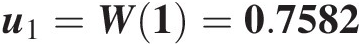
C(u2| U1 = u1) = 0.6289Cu2U1=u1=0.6289
C(u3| U1 = u1, U2 = u2) = 0.9611;Cu3U1=u1U2=u2=0.9611;
C(U4| U1 = u1, U2 = u2, U3 = u3) = 0.2743CU4U1=u1U2=u2U3=u3=0.2743.
2. Simulate u2u2 from C(U2| U1 = u1) = 0.6289CU2U1=u1=0.6289.
According to the fitted D-vine copula, we know [U1, U2]U1U2 is fitted with the BB1 copula (i.e., Equation (9.1)) with parameters [1.0203,1.9788]. Its conditional copula is then written as follows:
Cu2U1=u1=∂Cu1u2∂u1u1=0.6478=S1θ2−1u1−θ1−1θ2−1u1θ1+1S1θ2+11θ1+1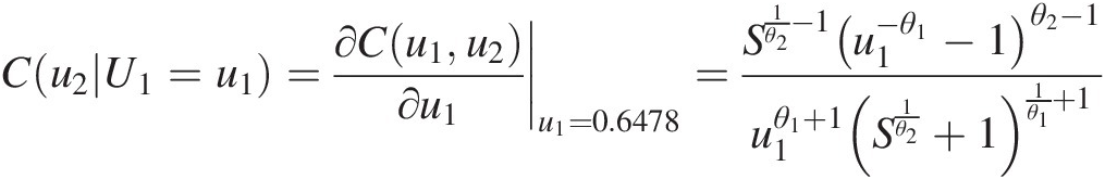 (10.7)
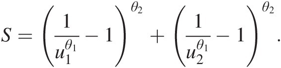
where:S=1u1θ1−1θ2+1u2θ1−1θ2.
Substituting u1 = 0.7582u1=0.7582 and C(u2| U1 = u1) = 0.6289Cu2U1=u1=0.6289 into Equation (10.7), we can solve for u2u2 numerically and obtain the following:
u2=0.7755.
3. Simulate u3u3 from C(u3| U1 = 0.7582, U2 = 0.7755)Cu3U1=0.7582U2=0.7755.
According to the fitted D-vine copula, we know U2U2 is the one of the center variables, and from the probability density composition discussed in Chapter 5, we have the following:
Cu3U1=u1U2=u2=∂C13∣2C3∣2C1∣2∂C1∣2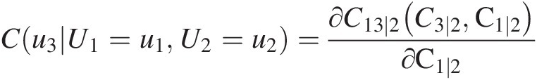 (10.8)
As seen in Equation (10.8), we may simulate u3u3 with the following two steps:
i. Compute C3 ∣ 2C3∣2 from C13 ∣ 2C13∣2. According to Figure 10.6, we know that the BB1 copula with parameter [0.2336, 1.0001] properly models C13 ∣ 2(C3 ∣ 2, C1 ∣ 2)C13∣2C3∣2C1∣2. With this in mind and after computing C1 ∣ 2C1∣2 using the BB1 conditional copula (i.e., Equation (10.7)), we immediately have the following: C(U1 ≤ 0.7582| U2 = 0.7755) = 0.5465CU1≤0.7582U2=0.7755=0.5465. Given {C3 ∣ 2, C1 ∣ 2}C3∣2C1∣2 (i.e., one of the bivariate copulas at T2) again modeled by the BB1 copula, C3 ∣ 2C3∣2 can then be computed by substituting C1 ∣ 2 = 0.5465C1∣2=0.5465 as u1u1 and C3 ∣ 2C3∣2 as u2u2, and by equating Equation (10.8) to 0.9383. We can solve for C3 ∣ 2C3∣2 numerically as C3 ∣ 2 = 0.9636C3∣2=0.9636.
ii. Compute u3u3 from C3 ∣ 2C3∣2. From Figure 10.6, {U2, U3}U2U3 is also modeled with the BB1 copula; u3u3 can then be solved for numerically by substituting u2 = 0.7755u2=0.7755 as u1u1, and u3u3 as u2u2 into Equation (10.7), and by setting the equation equal to C3 ∣ 2 = 0.9636C3∣2=0.9636. We then have the following:
u3=0.9383.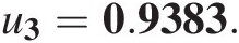
4. Simulate u4u4 from C(u4| U1 = 0.7582, U2 = 0.7755, U3 = 0.6865)Cu4U1=0.7582U2=0.7755U3=0.6865.
From the fitted D-vine copula, we know the conditional copula C(u4| U1 = u1, U2 = u2, U3 = u3)Cu4U1=u1U2=u2U3=u3 may be written using the probability function decomposition discussed in Chapter 5 as follows:
Cu4U1=u1U2=u2U3=u3=∂C14∣23C1∣23C4∣23∂C1∣23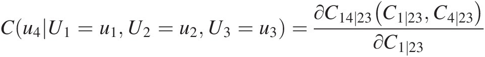 (10.9)
where:
C1∣23=∂C13∣2C1∣2C3∣2∂C3∣2;C4∣23=∂C24∣3C4∣3C2∣3∂C2∣3 (10.9a)
We know from Equations (10.9) and (10.9a) that C14 ∣ 23, C1 ∣ 23, and C4 ∣ 23C14∣23,C1∣23,andC4∣23 are modeled by bivariate Frank, BB1, and BB1 copulas, respectively (Figure 10.6). To this end, we can simulate u4u4 with the steps given in what follows:
i. Simulate C4 ∣ 23C4∣23 using C(u4| U1 = 0.75821, U2 = 0.7755, U3 = 0.9383) = 0.2743Cu4U1=0.75821U2=0.7755U3=0.9383=0.2743.
With the previously simulated u1, u2, u3u1,u2,u3, we first compute the conditional copula C1 ∣ 23C1∣23 in Equation (10.9a). Applying the corresponding fitted BB1 copulas, we compute the conditional copula as follows: C1 ∣ 2 = 0.5465, C3 ∣ 2 = 0.9636, C1 ∣ 23 = 0.4764C1∣2=0.5465,C3∣2=0.9636,C1∣23=0.4764. The given Frank copula may be applied to model C14 ∣ 23C14∣23 of T3, and Equation (10.9) may be rewritten using the conditional Frank copula as follows:
Cu4U1=u1U2=u2U3=u3=e−θC1∣23e−θC4∣23−1e−θC1∣23+C4∣23−e−θC1∣23−e−θC4∣23+e−θSubstituting θ = − 0.5062, C1 ∣ 23 = 0.4764, C(u4| U1 = u1, U2 = u2, U3 = u3) = 0.2743θ=−0.5062,C1∣23=0.4764,Cu4U1=u1U2=u2U3=u3=0.2743 into Equation (10.10), C4 ∣ 23C4∣23 is solved for numerically as follows: C4 ∣ 23 = 0.2777C4∣23=0.2777. (10.10)
ii. Simulate C4 ∣ 3C4∣3 using C(u4| U2 = 0.7755, U3 = 0.9383) = 0.2777Cu4U2=0.7755U3=0.9383=0.2777.
C4 ∣ 3C4∣3 can be simulated from the conditional copula C4 ∣ 23C4∣23 through C24 ∣ 3C24∣3, given as Equation (10.9a). C24 ∣ 3C24∣3 may be modeled with the bivariate BB1 copula through C4 ∣ 3, C2 ∣ 3C4∣3,C2∣3. Applying the BB1 copula to {U2, U3U2,U3}, we can easily compute C2 ∣ 3 = C(U2 ≤ 0.7755| U3 = 0.9383) = 0.1736C2∣3=CU2≤0.7755U3=0.9383=0.1736. In model construction (e.g., Figure 10.6), C24 ∣ 3C24∣3 is also modeled by the BB1 copula. Thus, we can solve for C4 ∣ 3C4∣3 numerically as C4 ∣ 3 = 0.1867C4∣3=0.1867.
iii. Simulate u4u4 using C4 ∣ 3 = 0.1867C4∣3=0.1867.
We know that {U3, U4U3,U4} is modeled with the Gumbel–Hougaard copula (Figure 10.6), as shown in Chapter 4; the conditional Gumbel–Hougaard copula can be written as follows:
Cu4U3=u3=−lnu3−1+θ(−lnu3)θ+−lnu4θ−1+1θu3exp−lnu3θ+−lnu4θ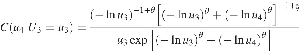 (10.11)
u4=0.6865


Finally, with four independent uniform random variables W = [0.7582, 0.6289, 0.9611, 0.2743]W=0.75820.62890.96110.2743; we successfully simulate the pseudo-rainfall variables from the fitted D-vine copula as follows:
Comparison of the simulated copula random variables with the pseudo-rainfall variables (the upper triangle of Figure 10.7) shows that the fitted D-vine copula reasonably preserves the overall dependence. With the use of 200 simulations, the lower triangle of Figure 10.7 compares the Kendall correlation coefficient computed from the simulations with the sample Kendall correlation coefficient computed from the observed four-dimensional rainfall variables. Comparison through the Kendall’s correlation coefficient indicates the following:
1. The sample correlation coefficient is within 50% bound for all free bivariate variates in T1, i.e.,
(U1, U2) : (R330058, R336949), (U2, U3) : (R336949, R333780), (U3, U4) : (R333780, R331358)U1U2:R330058R336949,U2U3:R336949R333780,U3U4:R333780R331358;
2. The sample correlation coefficient is also within 50% bound for the bivariate variates through conditioning, i.e., (U1, U3) : (R330058, R333780), (U1, U4) : (R330058, R331358)U1U3:R330058R333780,U1U4:R330058R331358.
3. The sample correlation coefficient is very close to the 50% bound for the last pair of the bivariate variate through conditioning: (U2, U4) : (R336949, R331358)U2U4:R336949R331358.
The preceding comparison ensures the appropriateness of applying the fitted D-vine copula model to investigate the four-dimensional rainfall variables. In addition, with the closeness of rain gauges, it is reasonable to assume that there may exist the tail dependence among the rainfall variables (i.e., there is the concurrent tendency of extreme weather events, e.g., storm events). The possible tail dependence makes the BB1 copula the best choice for a majority of cases. We will provide a detailed discussion in this regard when we compare the fitted vine copula to meta-elliptical and asymmetric Archimedean copulas later in the chapter.
10.3.2 Application of Meta-Elliptical Copula to Four-Dimensional Rainfall Variables
In this section, we will apply the meta-Gaussian and meta-Student t copula to model the four-dimensional rainfall variables. Using the same empirical marginals as those in Section 10.3.1, Table 10.11 lists the parameters (i.e., the correlation matrix for meta-Gaussian copula, and the correlation matrix and degree of freedom for meta-Student t copulas). With the estimated parameters, Figures 10.8 and 10.9 compare the simulated copula random variables with the pseudo-rainfall random variables as well as the simulated Kendall correlation coefficient with the sample Kendall correlation coefficient.
Table 10.11. Parameters estimated for meta-Gaussian and meta-Student t copulas.
| Stations | R330058 | R336949 | R333780 | R331358 | R330058 | R336949 | R333780 | R331358 |
|---|---|---|---|---|---|---|---|---|
| Meta-Gaussian copula | Meta-Student t copula | |||||||
| R330058 | 1 | 0.85 | 0.71 | 0.61 | 1 | 0.87 | 0.74 | 0.64 |
| R336949 | 0.85 | 1 | 0.75 | 0.72 | 0.87 | 1 | 0.78 | 0.74 |
| R333780 | 0.71 | 0.75 | 1 | 0.65 | 0.74 | 0.78 | 1 | 0.68 |
| R331358 | 0.61 | 0.72 | 0.65 | 1 | 0.64 | 0.74 | 0.68 | 1 |
| d.f. ν = 62.16ν=62.16 | ||||||||

Figure 10.8 Comparison with the fitted meta-Gaussian copula.

Simulations shown in Figures 10.8 and 10.9 indicate that the overall dependence structure of rainfall variables is very well preserved. In the case of overall dependence structure, the meta-Gaussian and meta-Student t copula visually perform better than the previously fitted D-vine copula, e.g., all sample Kendall correlation coefficients are within 50% bounds of the simulated Kendall correlation coefficients (200 simulations). Furthermore, the goodness-of-fit studies using the Rosenblatt transform yield the following:
Meta-Gaussian copula: SnB = 0.0245, P=SnB=0.0245,P=0.964.
Meta-Student t copula: SnB = 0.094, P = 0.785SnB=0.094,P=0.785.
10.3.3 Application of the Asymmetric Archimedean Copula to Four-Dimensional Rainfall Variables
In this section, we will evaluate the performance of asymmetric Archimedean copulas. Here we will choose the following two types of asymmetric structures (Figure 10.10). In Figure 10.10, U1, U2, U3, and U4 represent R330058, R336949, R333780, and R331358, respectively, as that applied for the D-vine and meta-elliptical copulas.

Figure 10.10 Asymmetric Archimedean copula structure.
As seen in Section 10.3.1, the BB1 and Gumbel–Hougaard copulas are found to properly model the bivariate random variables in T1. From Table 10.6, we see that the Gumbel–Hougaard copula comes to the second place to model (R330058, R336949), (R336949, R333780)R330058R336949,R336949R333780, and the BB1 copula comes as the second place to model (R333780, R331358)R333780,R331358). Given the possible difficulties to assess that the parameter of the higher level are lower than the parameter in the lower level (i.e., the parameter of C2 should be less than that of C1) for the two-parameter copulas, we will apply the second-best Gumbel–Hougaard copula for analysis. Applying the Gumbel–Hougaard copula and letting θ1, θ2, θ3θ1,θ2,θ3 represent the parameter for C1, C2, C3C1,C2,C3 respectively, the nested asymmetric Gumbel–Hougaard copula for the four-dimensional case can be written as follows:
 (10.12)
where θ1 ≥ θ2 ≥ θ3θ1≥θ2≥θ3
Table 10.12 lists the parameters as well as the Kendall correlation coefficient estimated for each level. The parameters listed in Table 10.12 fulfills the conditions for the nested asymmetric Archimedean copula (i.e., given as part of Equation (10.12)). Applying the goodness-of-fit study through the Rosenblatt transform, we obtain SnB = 0.048, P = 0.323.SnB=0.048,P=0.323. The goodness of fit results indicate the appropriateness of the fitted four-dimensional asymmetric Gumbel–Hougaard copula.
Table 10.12. Results from the nested asymmetric Gumbel–Hougaard copula.
| Parameters | C1 | C2 | C3 |
|---|---|---|---|
| θθ | 2.78 | 2.22 | 1.65 |
| ττ | 0.64 | 0.56 | 0.51 |
Furthermore, according to the discussion in Chapter 5, we may conclude that (i) pairs (R330058, R333780) and (R336949, R333780) should follow the Gumbel–Houggard copula with parameter θ2θ2; (ii) and pairs (R330058, R331358), (R336949, R331358), and (R333780, R331358) should all follow the Gumbel–Hougaard copula with parameter θ3θ3. Figure 10.11 compares the asymmetric Gumbel–Hougaard copula and bivariate Gumbel–Hougaard copula with the pseudo-observations. The scatter plots in Figure 10.11 show that the overall positive dependence may be captured; however, the box plots for the Kendall correlation coefficient indicate that (i) the sample Kendall correlation coefficient obviously falls out of the upper 50% bound for (R336949, R331358), and (R333780, R331358); (ii) the sample Kendall correlation coefficient is slightly higher than the upper 50% bound for (R336949, R333780); and (iii) the sample Kendall correlation coefficient is slightly higher than the 75% bound for (R336949, R331358).

Figure 10.11 Comparison of the asymmetric Gumbel–Hougaard copula with the pseudo-rainfall variables.
10.3.4 Comparison of D-vine, Meta-Elliptical, and Asymmetric Archimedean Copulas
In this section, we will compare the performances of fitted D-vine, meta-elliptical, and asymmetric Archimedean copulas for modeling the dependence in higher dimensions (i.e., four dimensions in this case study). Given all three types of fitted copulas passing the goodness-of-fit study, we will focus on the performance, freedom, and complexity of copula functions.
Flexibility and Complexity of Copula Functions
First, as discussed in Chapter 5, the vine copula is constructed, based on the probability density function decomposition, such that only bivariate copulas are considered as the building blocks either unconditionally (base level T1) or conditionally (upper levels). The bivariate copulas (i.e., the building blocks) are allowed for free specification (i.e., the copulas do not need to belong to the same family at all). Additionally, there are many choices for model construction. For example, in our four-dimension example illustrated here, we may be able to build 24 different D-vine copula structures through different pairing schemes.
Second, the meta-elliptical copula is only dependent on the correlation matrix for the meta-Gaussian copula, and the correlation matrix and degree of freedom for meta-Student t copula. In addition, its parameter estimation is easier than that of a vine copula.
Third, there are constraints on the asymmetric Archimedean copula. In addition, there are implications for the dependence for indirectly connected bivariate random variates (as discussed in the previous section).
Overall, the vine copula is most complex with the most flexibility of model construction. The meta-elliptical copula may always be able to capture the overall dependence. The asymmetric Archimedean copula has the least flexibility for model construction, and the dependence structure may not be properly captured due the theoretical constraints of the asymmetric copula function.
Comparison of Copula Performances
Applying Equation (5.61) in Chapter 5 to the fitted D-vine copula in Section 10.3.1, we will be able to compute the joint CDF for the four-dimensional rainfall variables. Similar to application of Equation (7.32) and Equation (7.46) in Chapter 7 and Equation (10.12), we can compute the joint CDF fitted by the meta-Gaussian, meta-Student t and asymmetric Gumbel–Hougaard copulas for the four-dimensional rainfall variables. Figure 10.12 compares the fitted parametric four-dimensional copula function with the nonparametric empirical copulas. Table 10.13 lists the RMSE computed between the parametric and empirical copulas. Figure 10.12 shows that (1) there is minimal visual difference between the performance of meta-Gaussian and that of meta-Student T copulas; (2) there is visual difference between the performance of fitted D-vine copula and asymmetric GH copula; and (3) the fitted D-vine copula may underestimate the JCDF for higher orders (>35) more than the asymmetric GH copula. The RMSE results listed in Table 10.13 further confirm the findings visually seen in Figure 10.12.

Figure 10.12 Comparison of vine, meta-elliptical, and asymmetric Archimedean copulas with empirical copula.
Table 10.13. RMSE computed between parametric and empirical copulas.
| Copula | D-vine | Asymmetric GH | Meta-Gaussian | Meta-Student t |
|---|---|---|---|---|
| RSME | 0.040 | 0.032 | 0.029 | 0.027 |
Comparing all three types of the copulas, one may directly apply the meta-elliptical copula for higher dimensions as the following:
1. The variance–covariance structure may be very well preserved (Figures 10.8 and 10.9).
2. A meta-elliptical copula is easy to construct, compared to both vine and asymmetric Archimedean copulas.
3. A meta-elliptical copula yields the overall best performance.
10.4 Summary
In this chapter, we discussed the application of copula to (1) the partial duration rainfall sequences to construct the DDF curve, and (2) the spatial dependence of precipitation measured from multiple rain gauge stations (i.e., four stations are selected in the case study).
The study shows the following:
i. Even with the differences between the NOAA and copula-based DDF curves constructed for the partial duration time series, the copula-based method may be considered as a rational alternative for rainfall DDF (or IDF) construction with simpler and faster rainfall separation (events regardless of the length of rainfall duration) compared to that of NOAA analysis (rainfall duration based directly).
ii. Applying vine, meta-elliptical, and asymmetric copulas to model the spatial dependence, we have found that the vine copula is most complex and most flexible at the same time. In regard to the copula performance, one may directly apply the meta-elliptical copula, given the simplicity of the parameter estimation and the capture of pairwise dependence structure for all correlated random variables.