Abstract
In this chapter, copula modeling is applied to flood analysis with the use of real-world flood data. The chapter is structured in the following sections: (i) an introduction; (ii) at-site flood frequency analysis; (iii) spatial dependence for flood variables; and (iv) concluding remarks.
11.1 Introduction
Univariate flood frequency analysis has long been done for design of hydraulic structures, such as levees, flood walls, spillways, dams, culverts, drainage structures, and reservoirs, as well as for risk and uncertainty analysis. In the past decade, hydrologists have employed the copula theory for bivariate/multivariate flood frequency analyses. The advantages of applying the copula theory are that (i) it allows for separate consideration of marginal distributions and the joint distribution (i.e., copulas); (ii) it allows one to investigate both linear and nonlinear dependence structures; (iii) the tail dependence may be better captured; and (iv) it is easier to extend to higher dimensions through the vine copula or meta-elliptical copulas. The copula methodology has been applied to model the bivariate and multivariate flood frequency analysis (Chowdhary et al., 2011; Chen et al., 2012, 2013; Bezak et al., 2014; Sraj et al., 2015; Durocher et al., 2016; Requena et al., 2016; among others).
11.2 At-Site Flood Frequency Analysis
Univariate flood frequency analysis (e.g., using annual peak discharge) has long been a standard hydrological design method. In the United States, the log-Pearson type III distribution is still the standard distribution for flood frequency analysis, even though it is known that annual peak discharge by itself is not sufficient to account for flood risk.
A given flood event may be characterized by three important characteristics, i.e., peak discharge, volume, and duration. These three characteristics interact with one another when assessing flood risk or flood damage. As an example, a flood event with a longer duration may breach a levee due to long inundation time and possibly a large flood volume, while the peak discharge in this case may not be high. Another example is when a flood event with a higher peak discharge and a shorter duration may overtop a flood wall, causing flood damage. To further explain how to do flood frequency analysis considering all three characteristics, we will use the flood data listed in Table 11.1 (Yue, 1999) as an illustrative example.
| Year | Q (cms) | V (day.cms) | D (days) | Year | Q (cms) | V (day.cms) | D (days) |
|---|---|---|---|---|---|---|---|
| 1963 | 968 | 58,538 | 111 | 1980 | 949 | 33,010 | 69 |
| 1964 | 1780 | 68,828 | 98 | 1981 | 1,500 | 64,631 | 114 |
| 1965 | 1330 | 38,682 | 73 | 1982 | 1,920 | 50,525 | 77 |
| 1966 | 1650 | 54,139 | 78 | 1983 | 1,590 | 67,223 | 80 |
| 1967 | 934 | 39,744 | 75 | 1984 | 1,460 | 57,769 | 96 |
| 1968 | 1100 | 37,213 | 84 | 1985 | 1,210 | 47,627 | 80 |
| 1969 | 1380 | 50,895 | 80 | 1986 | 1,690 | 46,735 | 74 |
| 1970 | 1780 | 66,879 | 96 | 1987 | 610 | 35,600 | 96 |
| 1971 | 1420 | 38,634 | 66 | 1988 | 993 | 36,882 | 80 |
| 1972 | 1160 | 42,497 | 79 | 1989 | 1,490 | 41,943 | 63 |
| 1973 | 1470 | 55,766 | 78 | 1990 | 1,570 | 38,568 | 59 |
| 1974 | 2400 | 84,198 | 80 | 1991 | 1,130 | 49,226 | 93 |
| 1975 | 1260 | 48,790 | 83 | 1992 | 1,820 | 51,752 | 77 |
| 1976 | 1490 | 60,767 | 84 | 1993 | 1,360 | 45,263 | 83 |
| 1977 | 1370 | 60,824 | 92 | 1994 | 1,170 | 74,840 | 126 |
| 1978 | 1530 | 63,663 | 102 | 1995 | 1,550 | 51,853 | 80 |
| 1979 | 2040 | 59,254 | 76 |
Note: a In this dataset, discharge (Q), flood volume (V), and flood duration (D) are considered independent identically distributed (i.i.d.) random variables.
The at-site trivariate flood frequency analysis in this chapter follows this procedure:
1. Collect the streamflow sequence and separate the streamflow sequence into peak discharge, flood duration, and flood volume variable.
2. Assess the pairwise overall dependence nonparametrically with the use of the Kendall rank-based correlation coefficient.
3. Apply the vine copula approach to study the dependence structure. The bivariate copula (building block) candidates are selected based on the nonparametric tail dependence coefficient and Kendall correlation coefficient.
4. Perform the risk analysis through the joint and conditional return period.
11.2.1 Brief Discussion of Dataset
As stated in Yue (1999), the flood dataset was collected for Asuapmushuan River basin in Quebec, Canada. Due to the constraints of the dataset, Yue (1999) applied the maximum annual daily discharge (Q [m3/s]), the corresponding flood volume (V [day m3/s]), and duration (D [day]) for frequency analysis. According to Yue (1999), the values of flood volume and duration were determined from the schematic (Figure 11.1) and Equation (11.1) as follows:
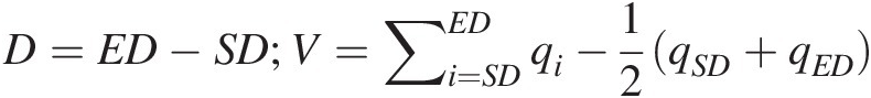 (11.1)
In Equation (11.1), SD and ED represent the starting time and the ending time of the flood event, respectively; D represents the duration of the flood event; qiqi represents the discharge of day-i during the flood event; and V represents the flood volume.
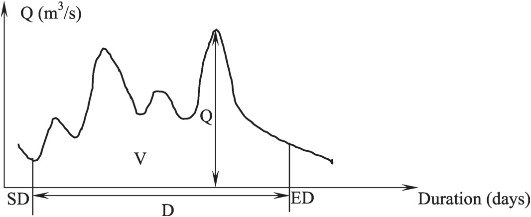
Figure 11.1 Schematic for a given flood event.
11.2.2 Dependence Measure of Flood Variables: Nonparametric Assessment
Before we apply copulas to at-site flood frequency analysis, we compute the sample Kendall’s correlation coefficient using Equation (3.73), as listed in Table 11.2. Using Equations (3.76)–(3.79) and Equation (3.80) presented in Sections 3.4.3 and 3.4.4, Figure 11.2 graphs the chi- and K-plots to assess the dependence among the flood random variables. Table 11.2 and Figure 11.2 clearly indicate the positive dependence between Q and V as well as between V and D, while the negative dependence is detected between Q and D. Physically, the dependence structure implies that (i) high flow tends to result in high flood volume; (ii) long flood duration (or long inundation time) also tends to lead to high flood volume (e.g., flood events due to slow moving storms); (iii) a high flow event may lead to a short-duration flood event (e.g., flash flooding caused by short-duration, high-intensity storms). Thus, it is more advantageous to take all three flood characteristics into consideration than assuming peak flow and flood duration being independent, as is usually done in conventional at-site bivariate/multivariate flood frequency analysis (e.g., Yue (1999)). In addition, the K-plots in the upper triangle of Figure 11.2 confirm the positive dependence of Q and V and of V and D and close to the independence of Q and D, the same as the chi-plots in the lower triangle and scatter plots of (Q, V), (V, D), and (Q, D) placed diagonally.

With the initial dependence assessment, we will apply the vine copula, meta-Gaussian, and meta-Student t copulas to model the dependence structure for trivariate flood variables.
11.2.3 Vine Copula–Based at-Site Flood Frequency Analysis
As discussed in Chapter 5, vine copulas belong to the asymmetric copula family. Given that flood volume has a higher degree of association with both flood peak flow and flood duration, we choose volume as the center variable to build the vine structure, as shown in Figure 11.3. As shown in Figure 11.3 and the discussions in Chapter 5, the bivariate copula is the building block for the entire structure. More specifically, we have full freedom to choose the best-fitted copula for (Q, V) and (V, D) separately in T1. Then, based on the best-fitted copula in T1 we will be able to choose the best-fitted copula in T2.

Figure 11.3 Vine-copula schematic for at-site trivariate flood variables.
Copula Candidates for T1
As shown in Figure 11.3 and the discussions in the previous chapters, we need to first compute the marginal distributions nonparametrically (e.g., Weibull plotting position formula Equation (3.103), or kernel density) or parametrically with fitted marginal distributions. Here we will use the Weibull plotting position formula to compute the marginals, as shown in Table 11.3. Before we choose the copula candidate, we assess the tail dependence of (Q, V) and (V, D) such that we can make a better judgment to choose the candidate. Figure 11.4 shows the scatter plot using the empirical marginals of each of (Q, V) and of each of (V, D). Compared to the left tail (i.e., the lower tail) dependence, we are usually more interested in the right tail (i.e., the upper tail) dependence for these extreme events. Based on the tail dependence concept discussed in Chapter 3, we will first introduce how to evaluate the empirical tail dependence coefficient in what follows.
Table 11.3. Marginal distributions computed using the Weibull plotting position formula.
| Year | Q (cms) | V (day cms) | D (days) | F(Q) | F(V) | F(D) |
|---|---|---|---|---|---|---|
| 1963 | 968 | 58,538 | 111 | 0.12 | 0.68 | 0.91 |
| 1964 | 1,780 | 68,828 | 98 | 0.84 | 0.91 | 0.85 |
| 1965 | 1,330 | 38,682 | 73 | 0.35 | 0.21 | 0.15 |
| 1966 | 1,650 | 54,139 | 78 | 0.76 | 0.59 | 0.34 |
| 1967 | 934 | 39,744 | 75 | 0.06 | 0.24 | 0.21 |
| 1968 | 1,100 | 37,213 | 84 | 0.18 | 0.12 | 0.66 |
| 1969 | 1,380 | 50,895 | 80 | 0.44 | 0.50 | 0.49 |
| 1970 | 1,780 | 66,879 | 96 | 0.84 | 0.85 | 0.79 |
| 1971 | 1,420 | 38,634 | 66 | 0.47 | 0.18 | 0.09 |
| 1972 | 1,160 | 42,497 | 79 | 0.24 | 0.29 | 0.38 |
| 1973 | 1,470 | 55,766 | 78 | 0.53 | 0.62 | 0.34 |
| 1974 | 2,400 | 84,198 | 80 | 0.97 | 0.97 | 0.49 |
| 1975 | 1,260 | 48,790 | 83 | 0.32 | 0.41 | 0.60 |
| 1976 | 1,490 | 60,767 | 84 | 0.57 | 0.74 | 0.66 |
| 1977 | 1,370 | 60,824 | 92 | 0.41 | 0.76 | 0.71 |
| 1978 | 1,530 | 63,663 | 102 | 0.65 | 0.79 | 0.88 |
| 1979 | 2,040 | 59,254 | 76 | 0.94 | 0.71 | 0.24 |
| 1980 | 949 | 33,010 | 69 | 0.09 | 0.03 | 0.12 |
| 1981 | 1,500 | 64,631 | 114 | 0.62 | 0.82 | 0.94 |
| 1982 | 1,920 | 50,525 | 77 | 0.91 | 0.47 | 0.28 |
| 1983 | 1,590 | 67,223 | 80 | 0.74 | 0.88 | 0.49 |
| 1984 | 1,460 | 57,769 | 96 | 0.50 | 0.65 | 0.79 |
| 1985 | 1,210 | 47,627 | 80 | 0.29 | 0.38 | 0.49 |
| 1986 | 1,690 | 46,735 | 74 | 0.79 | 0.35 | 0.18 |
| 1987 | 610 | 35,600 | 96 | 0.03 | 0.06 | 0.79 |
| 1988 | 993 | 36,882 | 80 | 0.15 | 0.09 | 0.49 |
| 1989 | 1,490 | 41,943 | 63 | 0.57 | 0.26 | 0.06 |
| 1990 | 1,570 | 38,568 | 59 | 0.71 | 0.15 | 0.03 |
| 1991 | 1,130 | 49,226 | 93 | 0.21 | 0.44 | 0.74 |
| 1992 | 1,820 | 51,752 | 77 | 0.88 | 0.53 | 0.28 |
| 1993 | 1,360 | 45,263 | 83 | 0.38 | 0.32 | 0.60 |
| 1994 | 1,170 | 74,840 | 126 | 0.26 | 0.94 | 0.97 |
| 1995 | 1,550 | 51,853 | 80 | 0.68 | 0.56 | 0.49 |

Figure 11.4 Scatter plots for the marginal of (Q, V) and of (V, D).
The tail dependence may be evaluated either graphically (Abberger, 2005) or numerically (Frahm et al., 2005; Schmidt and Stradtmuller, 2006). Here the nonparametric estimation is discussed in detail. Following Frahm et al. (2005), the nonparametric estimation is based on the empirical copula (i.e., Equation (3.64)) without any assumption on either parametric copula or marginals. In general, there are three types of nonparametric estimation (i.e., log-estimator [LOG], secant of the copula’s diagonal [SEC], and CFG; Poulin et al., 2007) for the upper-tail dependence (λ̂U ) that can be expressed as follows:
 (11.2)
 (11.3)
 (11.4)
In Equations (11.2)–(11.4), n is the sample size; Ui, Vi are the marginal variables; and k is the chosen threshold of the LOG and SEC methods.
The LOG method was proposed by Coles et al. (1999). The SEC method first appeared in Joe (1997). The threshold k can be estimated using the heuristic plateau-finding algorithm proposed by Frahm et al. (2005), which can be formulated as follows:
1. Smooth using the box kernel with bandwidth b ∈ ℕb∈ℕ (usually each moving average window should maintain 1% data) to compute the average of (2b + 1)2b+1 successive points from λ̂1,…,λ̂n
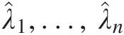 (i.e., mapping k↦λ̂k,k=1,2,…,n
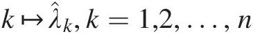 ) to obtain λ¯1,…,λ¯n−2b
 .
.
2. Set plateau length m=⌊n−2b⌋
 and define a vector: pk=λ¯k…λ¯k+m−1,k=1,…,n−2b−m+1.
3. Set the stopping criteria using the standard deviation of λ¯1,…,λ¯n−2b
 . The threshold k can then be estimated from the first plateau pkpk that satisfies the condition:
∑i=k+1k+m−1λ¯i−λ¯k≤2σ (11.5)
If k is un-identified, λ̂U
 is set as 0; otherwise, move on to step 4.
4. Estimate the upper-tail dependence coefficient for threshold k as follows:
λ̂Uk=1m∑i=1mλ¯k+i−1 (11.6)


The CFG method (i.e., Equation (11.4)) first appeared in Capéraà et al. (2007) that does not require the estimation of a threshold. However, there exists a strong underlying assumption: the empirical copula may be approximated by the extreme value (EV) copula (e.g., the Gumbel–Hougaard copula as an example). It is worth noting that the lower-tail dependence is the same as the upper-tail dependence of the survival copula.
The empirical upper-/lower-tail dependence coefficient is computed, as listed in Table 11.4. To illustrate the procedure, the empirical upper-tail dependence coefficient is further explained using Q and V with the LOG method. From the sample data listed in Table 11.1, the sample size is n = 33n=33. Applying Equation (11.2), we compute λ̂k for k = 1, 2, …, 32,k=1,2,…,32, as listed in Table 11.5. With the initial λ̂k
 s estimated for the LOG method, we can now move on to evaluate the tail dependence. With the sample size of 33, we set the bandwidth b = 0. With b = 0b=0, we have λ̂k=λ¯k
 , and the standard deviation of vector λ¯
 s is 0.2114. The plateau length m = 5 yields the vector with size of 27 by 5 for the non-NaN values that are listed in Table 11.6. Finally, applying Equation (11.5), we obtain the first p vector that satisfies the condition that index k = 3k=3 that results in the following:

We obtain the upper tail dependence as λULOG≈0.29 .
.
Table 11.4. Upper- and lower-tail dependence coefficients for (Q, V) and (V, D).
| Upper | Lower | ||||
|---|---|---|---|---|---|
| LOG | SEC | CFG | LOG | SEC | |
| Q & V | 0.29 | 0.38 | 0.43 | 0.74 | 0.95 |
| V & D | 0.49 | 0.60 | 0.51 | 0.60 | 0.92 |
Table 11.5. λ̂k computed using Equation (11.2).

| k | CmCm | λ̂k | k | CmCm | λ̂k |
|---|---|---|---|---|---|
| 1 | 0.9697 | 1.0000 | 17 | 0.3636 | 0.6026 |
| 2 | 0.9091 | 0.4755 | 18 | 0.3333 | 0.6066 |
| 3 | 0.8485 | 0.2761 | 19 | 0.3030 | 0.6076 |
| 4 | 0.7879 | 0.1549 | 20 | 0.2727 | 0.6053 |
| 5 | 0.7576 | 0.3102 | 21 | 0.2121 | 0.4672 |
| 6 | 0.7273 | 0.4131 | 22 | 0.1818 | 0.4483 |
| 7 | 0.6667 | 0.2993 | 23 | 0.1818 | 0.5721 |
| 8 | 0.6061 | 0.1963 | 24 | 0.1515 | 0.5476 |
| 9 | 0.5758 | 0.2664 | 25 | 0.1515 | 0.6683 |
| 10 | 0.5455 | 0.3210 | 26 | 0.1212 | 0.6391 |
| 11 | 0.4848 | 0.2146 | 27 | 0.1212 | 0.7622 |
| 12 | 0.4545 | 0.2556 | 28 | 0.0909 | 0.7293 |
| 13 | 0.4242 | 0.2878 | 29 | 0.0606 | 0.6715 |
| 14 | 0.3939 | 0.3126 | 30 | 0.0606 | 0.8309 |
| 15 | 0.3939 | 0.4631 | 31 | 0.0303 | 0.7527 |
| 16 | 0.3939 | 0.5956 | 32 | 0 |
Table 11.6. Vector p with the plateau length m = 5.
| k | λ¯k | λ¯k+1 | λ¯k+2 | λ¯k+3 | λ¯k+4 |
|---|---|---|---|---|---|
| 1 | 1.0000 | 0.4755 | 0.2761 | 0.1549 | 0.3102 |
| 2 | 0.4755 | 0.2761 | 0.1549 | 0.3102 | 0.4131 |
| 3 | 0.2761 | 0.1549 | 0.3102 | 0.4131 | 0.2993 |
| 4 | 0.1549 | 0.3102 | 0.4131 | 0.2993 | 0.1963 |
| 5 | 0.3102 | 0.4131 | 0.2993 | 0.1963 | 0.2664 |
| 6 | 0.4131 | 0.2993 | 0.1963 | 0.2664 | 0.3210 |
| 7 | 0.2993 | 0.1963 | 0.2664 | 0.3210 | 0.2146 |
| 8 | 0.1963 | 0.2664 | 0.3210 | 0.2146 | 0.2556 |
| 9 | 0.2664 | 0.3210 | 0.2146 | 0.2556 | 0.2878 |
| 10 | 0.3210 | 0.2146 | 0.2556 | 0.2878 | 0.3126 |
| 11 | 0.2146 | 0.2556 | 0.2878 | 0.3126 | 0.4631 |
| 12 | 0.2556 | 0.2878 | 0.3126 | 0.4631 | 0.5956 |
| 13 | 0.2878 | 0.3126 | 0.4631 | 0.5956 | 0.6026 |
| 14 | 0.3126 | 0.4631 | 0.5956 | 0.6026 | 0.6066 |
| 15 | 0.4631 | 0.5956 | 0.6026 | 0.6066 | 0.6076 |
| 16 | 0.5956 | 0.6026 | 0.6066 | 0.6076 | 0.6053 |
| 17 | 0.6026 | 0.6066 | 0.6076 | 0.6053 | 0.4672 |
| 18 | 0.6066 | 0.6076 | 0.6053 | 0.4672 | 0.4483 |
| 19 | 0.6076 | 0.6053 | 0.4672 | 0.4483 | 0.5721 |
| 20 | 0.6053 | 0.4672 | 0.4483 | 0.5721 | 0.5476 |
| 21 | 0.4672 | 0.4483 | 0.5721 | 0.5476 | 0.6683 |
| 22 | 0.4483 | 0.5721 | 0.5476 | 0.6683 | 0.6391 |
| 23 | 0.5721 | 0.5476 | 0.6683 | 0.6391 | 0.7622 |
| 24 | 0.5476 | 0.6683 | 0.6391 | 0.7622 | 0.7293 |
| 25 | 0.6683 | 0.6391 | 0.7622 | 0.7293 | 0.6715 |
| 26 | 0.6391 | 0.7622 | 0.7293 | 0.6715 | 0.8309 |
| 27 | 0.7622 | 0.7293 | 0.6715 | 0.8309 | 0.7527 |
From the tail dependence coefficients evaluated and listed in Table 11.4, it is seen that there exist both upper and lower tail dependences for the bivariate (Q, V) and (V, D) flood variables. To this end, we will have the following choices to investigate the dependence:
i. Use a mixed copula to model the bivariate flood variables.
ii. Use two-parameter copulas (Joe, 1997) to model the bivariate flood variables.
iii. Use copulas with upper-tail dependence to model the bivariate flood variables.
In theory, (a) all three approaches should be able to capture the overall dependence structure; (b) compared with approaches ii and iii, approach i may better capture both upper and tail dependences; (c) among the three approaches, parameter estimation for approach i is most complex; and (d) if we are only concerned with the upper-tail dependence, we may prefer approach iii. In what follows, we will discuss the copula candidates for all three approaches.
Approach i: Mixture Copula for Bivariate Variables
Following the discussion in Chapter 4, we introduce the Archimedean copula class. In this class, the Gumbel–Hougaard copula possesses the upper-tail dependence only (λU=2−21θGH ), while its survival copula possesses lower-tail dependence (λL=2−21θSGH)
 ; and the Clayton copula only possesses the lower-tail dependence (λL=2−1θC
 ). In addition, the Gumbel–Hougaard copula may only model the positive dependence, while the Clayton copula may model both positive and negative dependences. Following the discussion in Chapter 7, the meta-Gaussian copula, which is elliptical, has no tail dependence. Now through this approach, we will choose two candidates:
The Gumbel–Hougaard and Clayton copulas are listed in Chapter 4. The bivariate meta-Gaussian copula is expressed in Chapter 7. The survival Gumbel–Hougaard copula (CSGHCSGH) and its density function (cSGHcSGH) can be written as follows:
In Equations (11.7a) and (11.7b), θ : θ ≥ 1θ:θ≥1 represents the copula parameter to be estimated.
The corresponding mixture copula model may then be written as follows:
where θ = [θ1, θ2, θ3]θ=θ1θ2θ3. a1, a2, a3 ∈ [0, 1] : a1 + a2 + a3 = 1;a1,a2,a3∈01:a1+a2+a3=1; are the weight factors.
Approach ii: Two-Parameter Copulas for Bivariate Variables
As discussed in Joe (1997), the two-parameter Archimedean copulas may be capable of capturing both the overall dependence and the tail dependence. Following Joe (1997), we will briefly introduce BB1 BB4, and BB7 copulas.
BB1 Copula
 (11.9)
Its generating function and tail dependence function can be written as follows:
 (11.9a)
The BB1 copula can only be applied to model the positive dependence and may be considered as a two-parameter Archimedean copula. It possesses both upper- and lower-tail dependences. The limiting copulas are Gumbel–Hougaard copula (θ1→0θ1→0) and Clayton copula (θ2 = 1θ2=1). With the combination of the Gumbel–Hougaard and Clayton copulas, the BB1 copula is able to capture both upper- and lower-tail dependences in which the upper-tail dependence is independent of parameter θ1θ1.
BB4 Copula
 (11.10)
where θ1 ≥ 0, θ2>0.θ1≥0,θ2>0. Its tail dependence functions can be written as follows:
 (11.10a)
Unlike the BB1 copula, the BB4 copula is not a two-parameter Archimedean copula. Its limiting copulas are the Clayton copula when θ2→0θ2→0 and the Galambos copula when θ1→0θ1→0. The Glambos copula belongs to an extreme value copula given as follows:
 (11.10b)
As seen from Equation (11.10a), the upper-tail dependence of the BB4 copula is independent of parameter θ1.θ1.
BB7 Copula
 (11.11)
where θ1 ≥ 1, θ2>0θ1≥1,θ2>0.
BB7 is the same as the BB1 copula and is also a two-parameter Archimedean copula. Its generating function and tail dependence functions can be expressed as follows:
 (11.11a)
The limiting copulas for the BB7 copula are the Clayton copula when θ1 = 1θ1=1 and the Joe copula when θ2→0θ2→0.
Approach iii: Choosing Copulas with Upper-Tail Dependence
The copulas are chosen from the Archimedean, extreme, and elliptical copula families as follows:
Archimedean family: Gumbel–Hougaard and Joe copulas
Extreme copula family: Galambos copula
Elliptical copula family: meta-Student t copula, λU=λL=2tν+1−ν+11−ρ1+ρ
 .
.

Among the copulas listed in approach iii, all four copulas possess the upper-tail dependence. In addition, only the meta-Student t copula also possesses the symmetric lower-tail dependence.
Parameter Estimation and the Best-Fitted Copula for T1
Parameter Estimation for Approach i: Mixture Copula
The pseudo-MLE discussed in Chapter 4 is applied to estimate the parameters of the mixture copula. The initial parameters are set as follows:
✓ Each copula is of equal weight.
✓ The initial copula parameters are represented as the random variables, which may be modeled by one copula.
For each case, we have the following:
Q & V
Case (A):
a1 = 0.1652, θGH = 4.0597; a2 = 0.8348, θSGH = 1.6549, a3 = 0, θnormal = 0.5955.a1=0.1652,θGH=4.0597;a2=0.8348,θSGH=1.6549,a3=0,θnormal=0.5955.
LL=8.5657,AIC=−7.131;λU=0.13;λL=0.40.
Case (B):
a1 = 0.2295, θGH = 3.7289; a2 = 0.7705, θclayton = 1.1227; a3 = 0; θnormal = 0.5955a1=0.2295,θGH=3.7289;a2=0.7705,θclayton=1.1227;a3=0;θnormal=0.5955
LL=8.8470,AIC=−7.694;λU=0.1826;λL=0.4156


V & D
Case (A):
a1 = 0.7482, θGH = 2.0434; a2 = 0.2518, θSGH = 1.1900, a3 = 0, θnormal = 0.5845.a1=0.7482,θGH=2.0434;a2=0.2518,θSGH=1.1900,a3=0,θnormal=0.5845.
LL=6.7587,AIC=−3.5174;λU=0.446;λL=0.0528.
Case (B):
a1 = 0.7628, θGH = 2.0164; a2 = 0.2372, θclayton = 0.3963, a3 = 0, θnormal = 0.5845.a1=0.7628,θGH=2.0164;a2=0.2372,θclayton=0.3963,a3=0,θnormal=0.5845.
LL=6.7627,AIC=−3.525;λU=0.4499;λL=0.0413.


Parameter Estimation for Copula Candidates in Approaches ii and iii
Similar to approach i, the pseudo-MLE is applied to estimate the parameters for the copula candidates presented in approaches ii and iii, which are listed in Table 11.7.
Table 11.7. Results of two-parameter and one-parameter copula candidates for T1.
Considering the number of parameters, the overall dependence, and tail dependence, the BB7 copula is selected to model the dependence of Q & V as well as V & D for T1. To further ensure the appropriateness of the selected copula, the formal SnB test is performed. Based on Rosenblatt’s transform, the SnB
 test was introduced in Section 3.8.3. Hence, we have the following:

With the confirmation from the formal goodness-of-fit statistical test, we fix the copula in T1 and move on to T2.
Copula Selection for T2
To select the copula and estimate its parameters for T2, we first compute the conditional copula of Q ∣ VQ∣V and D ∣ VD∣V using the fitted BB7 copula for T1. The conditional copulas of Q|V and D|V are obtained by taking the partial derivative with respect to F(v)Fv that are listed in Table 11.8.
| Fn(Q)FnQ | Fn(V)FnV | Fn(D)FnD | FQV=∂CFnqFnv∂Fnv | FDV=∂CFndFnv∂Fnv |
|---|---|---|---|---|
| 0.12 | 0.68 | 0.91 | 0.02 | 0.95 |
| 0.84 | 0.91 | 0.85 | 0.57 | 0.54 |
| 0.35 | 0.21 | 0.15 | 0.59 | 0.22 |
| 0.76 | 0.59 | 0.34 | 0.78 | 0.26 |
| 0.06 | 0.24 | 0.21 | 0.04 | 0.30 |
| 0.18 | 0.12 | 0.66 | 0.47 | 0.90 |
| 0.44 | 0.50 | 0.49 | 0.39 | 0.50 |
| 0.84 | 0.85 | 0.79 | 0.69 | 0.58 |
| 0.47 | 0.18 | 0.09 | 0.77 | 0.14 |
| 0.24 | 0.29 | 0.38 | 0.27 | 0.50 |
| 0.53 | 0.62 | 0.34 | 0.42 | 0.24 |
| 0.97 | 0.97 | 0.49 | 0.78 | 0.05 |
| 0.32 | 0.41 | 0.60 | 0.30 | 0.71 |
| 0.57 | 0.74 | 0.66 | 0.39 | 0.54 |
| 0.41 | 0.76 | 0.71 | 0.18 | 0.58 |
| 0.65 | 0.79 | 0.88 | 0.44 | 0.85 |
| 0.94 | 0.71 | 0.24 | 0.96 | 0.11 |
| 0.09 | 0.03 | 0.12 | 0.67 | 0.49 |
| 0.62 | 0.82 | 0.94 | 0.37 | 0.94 |
| 0.91 | 0.47 | 0.28 | 0.96 | 0.25 |
| 0.74 | 0.88 | 0.49 | 0.45 | 0.17 |
| 0.50 | 0.65 | 0.79 | 0.36 | 0.82 |
| 0.29 | 0.38 | 0.49 | 0.28 | 0.58 |
| 0.79 | 0.35 | 0.18 | 0.90 | 0.18 |
| 0.03 | 0.06 | 0.79 | 0.11 | 0.97 |
| 0.15 | 0.09 | 0.49 | 0.50 | 0.80 |
| 0.57 | 0.26 | 0.06 | 0.77 | 0.06 |
| 0.71 | 0.15 | 0.03 | 0.94 | 0.05 |
| 0.21 | 0.44 | 0.74 | 0.13 | 0.84 |
| 0.88 | 0.53 | 0.28 | 0.93 | 0.23 |
| 0.38 | 0.32 | 0.60 | 0.47 | 0.75 |
| 0.26 | 0.94 | 0.97 | 0.03 | 0.89 |
| 0.68 | 0.56 | 0.49 | 0.67 | 0.46 |
Computing Kendall’s correlation coefficient, we have τ = − 0.5265τ=−0.5265. With the negative correlation, we will choose the Frank, meta-Gaussian, and meta-Student t copulas as the candidates for modeling. Applying pseudo-MLE to the marginals estimated from the conditional copulas of Q|V and D|V (i.e., columns 4 and 5) with the initial parameter estimated from the estimated Kendall’s correlation coefficient, we obtain
Frank: θ = − 5.655, LL = 10.705, AIC = − 19.411θ=−5.655,LL=10.705,AIC=−19.411
Meta-Gaussian: ρ = − 0.6898, LL = 10.656, AIC = − 19.3127ρ=−0.6898,LL=10.656,AIC=−19.3127
Meta-Student t: ρ = − 0.7034, ν = 17.4524; LL = − 10.776, AIC = − 17.553ρ=−0.7034,ν=17.4524;LL=10.776,AIC=−17.553
Based on the log-likelihood and AIC values, we choose Frank copula to model T2. Again applying the formal SnB goodness-of-fit test, we have the following: SnB=0.0456,P=0.207.
Now, we have finished building the vine-copula structure for the flood peak (Q), flood duration (D), and flood volume (V) variables in which the BB7 copula is applied to model the dependence of Q&V as well as of D&V in T1. The reasons we choose the BB7 copula are that (a) compared to the five-parameter mixture copula, the two-parameter BB7 copula reaches the smallest AIC value; and (b) the BB7 copula reasonably captures the tail dependence of Q&V as well as D&V. Figure 11.5 compares simulated random variates with pseudo-observations. In Figure 11.5 Kendall’s tau computed from simulation is also compared with sample Kendall’s tau: τQ, V = 0.41, τV, D = 0.42; τQ, D = − 0.13τQ,V=0.41,τV,D=0.42;τQ,D=−0.13. As seen in the box plots for (Q, V) and (V, D), the random variables simulated from the fitted BB7 copula well represent their dependence structure. Even though we did not directly investigate the copula function of (Q, D), the random variables simulated from the fitted BB7–BB7–Frank vine copula again reasonably represent the dependence structure of (Q, D).

Figure 11.5 Comparison of simulated variables with pseudo-observations.
11.2.4 At-Site Flood Risk Analysis
Similar to Yue et al. (1999), the Gumbel distribution is applied to model the marginal distributions for flood peak, volume, and duration to assess and compare the risk measure. The Gumbel distribution (also called the EV1 distribution) can be given as follows:
 (11.12)
where μx, αxμx,αx are, respectively, the location and the scale parameters for random variable X.
Using MLE, parameters of the marginal distributions are listed in Table 11.9. Figure 11.6 plots the frequency histograms for flood variables. Figure 11.6 shows that Gumbel distribution may not be the proper choice for flood duration. We further choose the log-normal distribution for flood duration. The parameters are also listed in Table 11.9.
Table 11.9. Fitted parametric marginal distributions and KS test results.
| Distribution | Discharge | Volume | Duration | |||
|---|---|---|---|---|---|---|
| Parameters | KS testa | Parameters | KS test | Parameters | KS test | |
| Gumbel | [1608.5, 383.9] | [0.14, 0.47] | [58591, 13148] | [0.13, 0.56] | [92.04, 16.89] | [0.23, 0.04] |
| Log-normal | [4.42, 0.17] | [0.17, 0.24] | ||||
Note: a In the KS test, the first column is the test statistics, the second column is the P-value.

Figure 11.6 Frequency histograms for the fitted Gumbel and log-normal distributions.
Joint and Conditional Return Periods for Bivariate Cases of Discharge and Flood Volume, and Flood Volume and Duration
In this section, we will discuss the important risk measure by using joint and conditional return periods for the bivariate case. For the joint return period, we will consider the “AND” and “OR” cases. For the conditional return period, we will consider the X>x ∣ Y>yX>x∣Y>y (e.g., Q>q ∣ V>v)Q>q∣V>v) and X>x ∣ Y = yX>x∣Y=y (e.g., the Q>q ∣ V = v)Q>q∣V=v) cases.
Joint Return Period of Discharge and Flood Volume, and Flood Volume and Duration
As discussed in Section 3.10.2, the joint return periods are computed for two cases: the “AND” case and “OR” case. In the “AND” case, the critical values set for both variables are exceeded. In the “OR” case, the critical value for at least one variable is exceeded. Using the 5-, 10-, 25-, 50-, 100-year discharge and flood volume events as criteria, we can easily compute the joint return period with the use of the BB7 copula fitted to the flood discharge and flood volume. The design events are listed in Table 11.10 for flood discharge (Q) and flood volume (V) with given return periods using the fitted parametric Gumbel distribution.
Table 11.10. Marginal design events with given return periods.
| Variables | Marginal | Return period (years) | ||||
|---|---|---|---|---|---|---|
| 5 | 10 | 25 | 50 | 100 | ||
| Discharge (cms) | Gumbel | 1,791.14 | 1,928.62 | 2,057.21 | 2,132.07 | 2,194.69 |
| Volume (cms·day) | Gumbel | 64,848.11 | 69,557.12 | 73,961.78 | 76,525.99 | 78,670.80 |
| Duration (day) | Log-normal | 95.57 | 102.78 | 111.06 | 116.76 | 122.14 |
| Gumbel | 100.08 | 106.13 | 111.79 | 115.08 | 117.84 | |
“AND” Case: T(V>v ∩ D>d)TV>v∩D>d
From Equation (3.136), the “AND” case implies to compute the survival copula of the bivariate random variable. using the five-year design discharge and the five-year design flood volume as an example, we can write the following:

With the same logic, the joint return periods of the “AND” case for Q&V and V&D are computed, as listed in Table 11.11.
Table 11.11. Joint return period of the “AND” case.
| Return period (years) | V (cms·day) | |||||
|---|---|---|---|---|---|---|
| 64848.11 | 69557.12 | 73961.78 | 76525.99 | 78670.80 | ||
| 1,791.14 | 9.68 | 15.54 | 32.33 | 59.40 | 112.37 | |
| Q (cms) | 1,928.62 | 15.54 | 21.78 | 39.29 | 67.40 | 122.04 |
| 2,057.21 | 32.33 | 39.29 | 57.56 | 86.74 | 143.61 | |
| 2,132.07 | 59.40 | 67.40 | 86.74 | 116.59 | 174.80 | |
| 2,194.69 | 112.37 | 122.04 | 143.61 | 174.80 | 234.21 | |
| D (day) | ||||||
|---|---|---|---|---|---|---|
| 95.57 | 102.78 | 111.06 | 116.76 | 122.14 | ||
| 64,848.11 | 8.76 | 13.68 | 28.78 | 54.03 | 104.39 | |
| 69,557.12 | 13.68 | 18.25 | 32.93 | 58.10 | 108.59 | |
| V (cms·day) | 73,961.78 | 28.78 | 32.93 | 46.24 | 70.38 | 120.45 |
| 76,525.99 | 54.03 | 58.10 | 70.38 | 92.69 | 140.92 | |
| 78,670.80 | 104.39 | 108.59 | 120.45 | 140.92 | 185.50 | |
“OR” Case: T(Q>q ∪ V>v)TQ>q∪V>v
The “OR” case implies that at least one variable exceeds the critical design value. The return period of the “OR” case is given in Equation (3.137). Using the five-year design discharge and the five-year design flood volume as an example, the exceedance probability of the “OR” case can be written as follows:

The rest of the “OR’ case computations are listed in Table 11.12.
Table 11.12. Joint return period of “OR” case.
| Return period (years) | V (cms·day) | |||||
|---|---|---|---|---|---|---|
| 64848.11 | 69557.12 | 73961.78 | 76525.99 | 78670.80 | ||
| 1,791.14 | 3.37 | 4.24 | 4.78 | 4.92 | 4.97 | |
| Q (cms) | 1,928.62 | 4.24 | 6.49 | 8.73 | 9.51 | 9.82 |
| 2,057.21 | 4.78 | 8.73 | 15.97 | 20.63 | 23.24 | |
| 2,132.07 | 4.92 | 9.51 | 20.63 | 31.82 | 41.19 | |
| 2,194.69 | 4.97 | 9.82 | 23.24 | 41.19 | 63.57 | |
| D (day) | ||||||
|---|---|---|---|---|---|---|
| 95.57 | 102.78 | 111.06 | 116.76 | 122.14 | ||
| 6,4848.11 | 3.50 | 4.41 | 4.87 | 4.96 | 4.99 | |
| 69,557.12 | 4.41 | 6.89 | 9.12 | 9.73 | 9.92 | |
| V (cms.day) | 73,961.78 | 4.87 | 9.12 | 17.13 | 21.84 | 23.98 |
| 76,525.99 | 4.96 | 9.73 | 21.84 | 34.23 | 43.66 | |
| 78,670.80 | 4.99 | 9.92 | 23.98 | 43.66 | 68.45 | |
Compared with the “AND” case, the return period of the “OR” case is less than that of the “AND” case. It is obviously in agreement with reality. As an example, the discharge may be exceeded, while the volume does not exceed the design volume and vice versa.
Conditional Return Period for Flood Discharge and Flood Volume, and Flood Volume and Flood Duration
In this section, we will discuss two cases of conditional return periods: (i) X>x ∣ Y>yX>x∣Y>y and (ii) X>x ∣ Y = yX>x∣Y=y.
Case i: T(X>x| Y>y)TX>xY>y
Following Nelsen (2006) as well as the discussion in Chapter 3, the conditional probability of P(X>x| Y>y) or C(FX>u| FY>v)PX>xY>yorCFX>uFY>v may lead to the right tail increasing (RTI) property, if 1−u−v+Cuv1−v is nondecreasing in u.
The return period is written with μ = 1μ=1 as follows:
 (11.13)
Using the flood volume as a conditioning variable, the conditional distribution and conditional return period are computed, as listed in Table 11.13. Figure 11.7 plots the conditional probability given V>vV>v for flood discharge and flood duration computed using the copula. Table 11.13 and Figure 11.7 show that the RTI property does exist for Q & V as well as V & D. The existence of RTI also implies the right tail dependence.
| Return period (years) | Given V > v (cms·day) | |||||
|---|---|---|---|---|---|---|
| 64848.11 | 69557.12 | 73961.78 | 76525.99 | 78670.80 | ||
| 1,791.14 | 48.41 | 77.72 | 161.63 | 297.02 | 561.84 | |
| Q (cms) | 1,928.62 | 155.44 | 217.83 | 392.86 | 673.97 | 1,220.36 |
| 2,057.21 | 808.16 | 982.16 | 1,439.00 | 2,168.49 | 3,590.12 | |
| 2,132.07 | 2,970.17 | 3,369.86 | 4,336.98 | 5,829.03 | 8,739.74 | |
| 2,194.69 | 11,236.71 | 12,203.58 | 14,360.48 | 17,479.48 | 23,419.82 | |
| Given D > d (day) | ||||||
|---|---|---|---|---|---|---|
| 95.57 | 102.78 | 111.06 | 116.76 | 122.14 | ||
| 64,848.11 | 95.57 | 102.78 | 111.06 | 116.76 | 122.14 | |
| 69,557.12 | 43.81 | 68.38 | 143.90 | 270.13 | 521.96 | |
| V (cms·day) | 73,961.78 | 136.75 | 182.47 | 329.27 | 580.97 | 1,085.94 |
| 76,525.99 | 719.48 | 823.17 | 1,155.97 | 1,759.44 | 3,011.34 | |
| 78,670.80 | 2,701.34 | 2,904.83 | 3,518.89 | 4,634.37 | 7,046.14 | |

Figure 11.7 Conditional probability plot for discharge and duration given that the flood volume is greater than the given threshold.
Case (ii): T(X>x| Y = y)TX>xY=y.
Following Nelsen (2006) and the discussion in Chapter 3, the conditional probability of P(X>x| Y = y)PX>xY=y or equivalently C(U>u| V = v)CU>uV=v may lead to stochastic monotonicity (or stochastic increasing of X in Y), i.e., ∂C(u, v)/∂v∂Cuv/∂v is a nonincreasing function in v. Or in other words, 1 − ∂C(u, v)/∂v1−∂Cuv/∂v is a nondecreasing function in v. For the chosen BB7 copula (i.e., Equation (11.11)), its partial derivative can be written as follows:
 (11.14)
Figure 11.8 plots the conditional probability of discharge given flood volume as well as flood duration given flood volume. Figure 11.8 clearly shows that discharge and duration are nonincreasing in flood volume. In other words, discharge and duration are stochastically increasing on flood volume and vice versa. As an example, under the conditions of V = {64848, 69557, 73926, 76526, 78670} cmsdayV=6484869557739267652678670cmsday, the conditional probability of P(Q>1500 cms| V = vi)PQ>1500cmsV=vi and P(D>90 day ∣ V = viP(D>90day∣V=vi) decreases as V increases. Figure 11.9 plots the conditional return period for given flood volume of Case ii using the following:
 (11.15)
Similar to Figure 11.8, Figure 11.9 also shows that under given flood volume (i.e., V = v), the higher discharge and longer duration result in a shorter return period and vice versa.

Figure 11.8 Conditional probability of flood discharge and duration for the given flood volume.

Figure 11.9 Conditional return period of flood discharge and duration for the given flood volume.
Comparing the results of the univariate return period, the joint return period (“OR” and “AND” cases), and the conditional return periods (Q>q|V>v, V>v|D>dQ>qV>vV>vD>d), the same conclusion (Serinaldi, 2015) is obtained, as follows:
11.2.5 Joint and Conditional Return Periods of Flood Discharge, Flood Volume and Flood Duration (Trivariate Case)
Similar to the bivariate case discussed in the previous sections, we will again consider the “AND” and “OR” cases for the joint return period. We will consider the following cases for the conditional return periods: (i)X>x ∪ Y>y ∣ Z>z (ii) X>x ∪ Y>y|Z = z, (iii) X>x ∩ Y>y| Z>z, (iv) X>x ∩ Y>y|Z = z, (v)X>x|Y>y, Z>z, (vi)X>x|Y = y, Z = ziX>x∪Y>y∣Z>ziiX>x∪Y>yZ=ziiiX>x∩Y>yZ>zivX>x∩Y>yZ=z,vX>xY>yZ>zviX>xY=y,Z=z As shown in Equation (5.60), the joint probability distribution of flood discharge (Q), flood volume (V), and flood duration (D) may be expressed through the conditional probability distribution as follows:
 (11.16)
In Equation (11.16), CQD ∣ V, CQ ∣ V, CD ∣ VCQD∣V,CQ∣V,CD∣V are fitted using Frank, BB7, and BB7 copulas, respectively. In Section 11.2.3, we have shown that such a fitted vine copula may properly represent the trivariate dependence structure for the trivariate flood variables using a formal goodness-of-fit test. Figure 11.10 graphically illustrates the appropriateness through the joint probability plot by ordered pair. In what follows, we will discuss the joint return periods first, followed by the conditional return periods.

Figure 11.10 Joint CDF plot for flood variables.
Joint Return Period of Flood Discharge, Flood Volume, and Flood Duration
“AND” Case: T(Q>q ∩ V>v ∩ D>d)TQ>q∩V>v∩D>d
As introduced in Chapter 3, the joint return period of the “AND” case may be expressed using Equation (3.149), which implies that flood discharge, flood volume, and flood duration all exceed their threshold values. To estimate the joint return period for the “AND” case, we need to know the bivariate joint distribution of flood discharge and flood duration. From the fitted vine copula structure, there does not exist a direct connection between flood discharge and flood duration; however, they are indirectly connected through flood volume. From Nelsen (2006) and the copula properties discussed in Chapter 3, we evaluate the joint distribution of flood discharge and duration by setting the marginal CDF for flood volume as 1, i.e.,
 (11.17)
Using the fitted BB7–BB7–Frank vine copula, Equation (11.17) is further reduced to integrating the conditional frank copula. Figure 11.10 also compares the empirical distribution with the parametric distribution derived from the fitted vine copula.
Table 11.14 shows the joint return period for the “AND” case using D = 90 daysD=90days as the threshold of flood duration for 5-, 10-, 25-, 50-, and 100-year design flood discharges and flood volumes.
“OR” Case: T(Q>q ∪ V>v ∪ D>d)TQ>q∪V>v∪D>d
As discussed in Chapter 3, at least one variable exceeds the threshold value. The joint return period is computed using Equation (3.150) for the “OR” case, that is, Q>q ∪ V>v ∪ D>dQ>q∪V>v∪D>d. As in the “AND” case, D = 90 daysD=90days is applied as the fixed threshold for flood duration. Table 11.14 also lists the computed “OR” case joint return period using the 5-, 10-, 25-, 50-, and 100-year design flood discharge and flood volume values as threshold values.
Table 11.14. Joint return period for trivariate flood variables (D = 90 days).
| Return period (years) | V (cms·day) “AND” case | |||||
|---|---|---|---|---|---|---|
| 64,848.11 | 69,557.12 | 73,961.78 | 76,525.99 | 78,670.80 | ||
| 1,791.14 | 15.96 | 16.30 | 16.77 | 17.03 | 17.20 | |
| Q (cms) | 1,928.62 | 27.02 | 27.32 | 27.79 | 28.09 | 28.29 |
| 2,057.21 | 52.95 | 53.23 | 53.74 | 54.14 | 54.48 | |
| 2,132.07 | 89.73 | 90.01 | 90.55 | 91.05 | 91.55 | |
| 2,194.69 | 156.13 | 156.42 | 157.01 | 157.61 | 158.31 | |
| V (cms·day) “OR” CASE | ||||||
|---|---|---|---|---|---|---|
| 64,848.11 | 69,557.12 | 73,961.78 | 76,525.99 | 78,670.80 | ||
| 1,791.14 | 2.13 | 2.14 | 2.06 | 2.02 | 1.99 | |
| 1,928.62 | 2.45 | 2.59 | 2.55 | 2.50 | 2.46 | |
| Q (cms) | 2,057.21 | 2.61 | 2.88 | 2.93 | 2.90 | 2.87 |
| 2,132.07 | 2.65 | 2.96 | 3.05 | 3.04 | 3.02 | |
| 2,194.69 | 2.67 | 2.98 | 3.10 | 3.11 | 3.10 | |
Figure 11.11 plots the joint return periods for the “AND” and “OR” cases. Figure 11.11 and Table 11.14 indicate that the risk of all three flood variables exceeding the threshold values is significantly smaller than at least one of the variables exceeding its threshold value.

Figure 11.11 Joint return periods for trivariate flood variables: “AND” and “OR” cases.
Conditional Return Periods of Flood Discharge, Volume, and Duration
As stated earlier, we are going to evaluate six different types of conditional return periods for flood discharge, volume, and duration. In traditional flood frequency analysis, the standard approach is to investigate the discharge variable only. Thus, in all six cases, we will consider discharge as one conditional variable.
Cases I and II: T(Q>q ∪ V>v| D>d)TQ>q∪V>vD>d; T(Q>q ∪ V>v| D = d)TQ>q∪V>vD=d
For case I, its conditional probability P(Q>q ∪ V>v| D>d)PQ>q∪V>vD>d can be derived as follows:
 (11.18b)
 (11.18c)
Following the same logic as that discussed for the bivariate case in Serinaldi (2015), the conditional return period of T(Q>q ∪ V>v| D>d)TQ>q∪V>vD>d can be written as follows:
 (11.18d)
For case II, i.e., T(Q>q ∪ V>v| D = d)TQ>q∪V>vD=d, its conditional probability of Q>q ∪ V>v ∣ D = dQ>q∪V>v∣D=d can be written as follows:
 (11.19a)
and
 (11.19b)
Applying the BB7–BB7–Frank copula to Equations (11.18) and (11.19), the conditional return periods are computed, as listed in Table 11.15, using five design flood discharge values and flood volume values as threshold values with the flood duration threshold value set as 90 days for exceedance (case I) and conditioning (case II). As shown in the preceding equations, in both of the cases at least one of the flood discharge or flood volume values exceeds its threshold value. Table 11.15 shows that higher conditional periods are obtained for case I than those for case II. Using the fitted log-normal distribution, the marginal probability FD(D ≤ 90) = 0.68FDD≤90=0.68. In general, the flood event with this duration occurs once in about three years. It is more likely for the large discharge or flood volume to occur for case I compared to case II. Figure 11.12 shows the conditional return periods for cases I and II of trivariate flood variables.
Table 11.15. Conditional return period for cases I and II.
| Return period (years) | V (cms·day) Q>q ∪ V>v ∣ D>d (90 days)Q>q∪V>v∣D>d90days | |||||
|---|---|---|---|---|---|---|
| 64,848.11 | 69,557.12 | 73,961.78 | 76,525.99 | 78,670.80 | ||
| 1,791.14 | 3.82 | 4.11 | 4.36 | 4.47 | 4.52 | |
| Q (cms) | 1,928.62 | 3.82 | 4.12 | 4.38 | 4.49 | 4.55 |
| 2,057.21 | 3.82 | 4.12 | 4.39 | 4.49 | 4.55 | |
| 2,132.07 | 3.82 | 4.12 | 4.39 | 4.50 | 4.56 | |
| 2,194.69 | 3.82 | 4.12 | 4.39 | 4.50 | 4.56 | |
| V (cms·day) Q>q ∪ V>v ∣ D = d (90 days)Q>q∪V>v∣D=d90days | ||||||
|---|---|---|---|---|---|---|
| 64,848.11 | 69,557.12 | 73,961.78 | 76,525.99 | 78,670.80 | ||
| 1,791.14 | 4.92 | 12.29 | 23.65 | 25.67 | 25.18 | |
| 1,928.62 | 5.09 | 14.65 | 45.16 | 63.63 | 67.72 | |
| Q (cms) | 2,057.21 | 5.15 | 15.66 | 67.30 | 143.75 | 193.39 |
| 2,132.07 | 5.16 | 15.88 | 75.66 | 207.61 | 370.12 | |
| 2,194.69 | 5.16 | 15.96 | 79.23 | 251.33 | 603.00 | |

Figure 11.12 Conditional return periods for cases I and II of trivariate flood variables.
Cases III and IV: T(Q>q ∩ V>v| D>d); T(Q>q ∩ V>v| D = d)TQ>q∩V>vD>d;TQ>q∩V>vD=d
For case III, i.e., T(Q>q ∩ V>v| D>d)TQ>q∩V>vD>d; its corresponding exceedance conditional probability can be written as follows:
 (11.20a)
Substituting Equation (3.136) with the copula from Chapter 3 into Equation (11.20a), we can rewrite Equation (11.20a) as follows:
 (11.20b)
Again, following the logic in Serinaldi (2015), the conditional return period can then be given as follows:
 (11.20c)
For case IV, i.e. T(Q>q ∩ V>v| D = d)TQ>q∩V>vD=d; its corresponding exceedance conditional probability can be written as follows:
 (11.21a)
The conditional return period can then be given as follows:
 (11.21b)
In Equation (11.21), PQ≤qD=d=∂CQD∂FDd with the joint distribution of flood discharge and duration derived in Equation (11.17).
Applying the fitted BB7–BB7–Frank vine copula, we compute the conditional return periods for the design events of discharge and flood volume using D = 90 days as the threshold value for flood duration. Table 11.16 lists the conditional return period computed for cases III and IV, and Figure 11.13 plots the conditional return periods. Compared to cases I and II, it is seen that the conditional return period computed for cases III and IV is much higher. The results confirm the real-world situation, that is, it is much harder for both flood discharge and flood volume to exceed the threshold values concurrently.
Table 11.16. Conditional return period for cases III and IV.
| Return period (years) | V (cms·day) Q>q ∩ V>v ∣ D>d (90 days)Q>q∩V>v∣D>d90days | |||||
|---|---|---|---|---|---|---|
| 64,848.11 | 69,557.12 | 73,961.78 | 76525.99 | 78670.80 | ||
| 1791.14 | 606.85 | 811.67 | 1,459.08 | 2,535.62 | 4,663.29 | |
| Q (cms) | 1928.62 | 1,584.71 | 1,993.04 | 3,273.31 | 5,396.37 | 9,570.15 |
| 2057.21 | 4,486.15 | 5,217.81 | 7,385.68 | 10,931.92 | 17,886.38 | |
| 2132.07 | 9,212.59 | 10,234.36 | 13,039.06 | 17,435.98 | 26,007.61 | |
| 2194.69 | 18,526.45 | 19,913.44 | 23,434.22 | 28,573.04 | 38,283.46 | |
| V (cms·day) Q>q ∩ V>v ∣ D = d (90 days)Q>q∩V>v∣D=d90days | ||||||
|---|---|---|---|---|---|---|
| 64,848.11 | 69557.12 | 73961.78 | 76525.99 | 78,670.80 | ||
| 1791.14 | 30.17 | 42.27 | 79.65 | 141.22 | 262.49 | |
| 1928.62 | 76.89 | 99.76 | 168.91 | 282.02 | 503.34 | |
| Q (cms) | 2057.21 | 214.06 | 253.33 | 363.83 | 541.51 | 888.36 |
| 2132.07 | 436.19 | 489.90 | 628.74 | 842.38 | 1,257.44 | |
| 2194.69 | 872.64 | 944.54 | 1,115.45 | 1,360.10 | 1,821.49 | |

Figure 11.13 Conditional return period plots for cases III and IV.
Cases V and VI: T(Q>q| V>v, D>d); T(Q>q| V = v, D = d)TQ>qV>vD>d;TQ>qV=vD=d
For case V, the conditional probability may be written as follows:
 (11.22a)
Using the same approach as described in Serinaldi (2015), its conditional return period can be given as follows:
 (11.22b)
For case VI, its conditional probability may be written as follows:
 (11.23b)
The conditional return periods computed for cases V and VI are tabulated and plotted in Table 11.17 and Figure 11.14, respectively. Table 11.17 indicates that higher conditional return periods are obtained for case V under the condition that V>vi ∩ D>90 daysV>vi∩D>90days than those for case VI under the condition that V = vi ∩ D = 90 daysV=vi∩D=90days. It is also seen that the conditional return period decreases for Q>qiQ>qi with the increase of flood volume for case VI. This result again agrees with the right tail dependence between flood discharge and flood volume. Compared to low discharge, high discharge is more likely to occur under the condition of high flood volume.
Table 11.17. Conditional return period for cases V and VI.
| Return period (years) | V (cms·day) Q>q ∣ V>v, D>d (90 days)Q>q∣V>v,D>d90days | |||||
|---|---|---|---|---|---|---|
| 64,848.11 | 69,557.12 | 73,961.78 | 76,525.99 | 78,670.80 | ||
| 1,791.14 | 1,344.57 | 3,090.00 | 1.25E+04 | 4.20E+04 | 1.51E+05 | |
| Q (cms) | 1,928.62 | 3,511.13 | 7,587.46 | 2.82E+04 | 8.94E+04 | 3.11E+05 |
| 2,057.21 | 9,939.68 | 1.99E+04 | 6.35E+04 | 1.81E+05 | 5.81E+05 | |
| 2,132.07 | 2.04E+04 | 3.90E+04 | 1.12E+05 | 2.89E+05 | 8.44E+05 | |
| 2,194.69 | 4.10E+04 | 7.58E+04 | 2.02E+05 | 4.73E+05 | 1.24E+06 | |
| V (cms·day) Q>q ∣ V = vD = d (90 days)Q>q∣V=vD=d90days | ||||||
|---|---|---|---|---|---|---|
| 64,848.11 | 69,557.12 | 73,961.78 | 76,525.99 | 78,670.80 | ||
| 1,791.14 | 4.04 | 1.38 | 1.05 | 1.02 | 1.01 | |
| 1,928.62 | 14.66 | 2.70 | 1.17 | 1.05 | 1.02 | |
| Q (cms) | 2,057.21 | 68.92 | 10.09 | 1.89 | 1.20 | 1.06 |
| 2,132.07 | 206.03 | 29.26 | 3.94 | 1.66 | 1.17 | |
| 2,194.69 | 601.85 | 84.80 | 10.04 | 3.12 | 1.55 | |

Figure 11.14 Conditional return period plots for cases V and VI.
11.2.6 Comparison with the Yue et al. (1999) Results
Compared with the results in Yue et al. (1999), there are some major differences for the case study presented using the same data listed in Yue et al. (1999). First, Yue, et al. (1999) applied the Gumbel (EV1) distribution as the marginal distribution for flood discharge, volume, and duration. According to the univariate goodness-of-fit test (i.e., the KS test), Table 11.9 shows the Gumbel distribution is proper for flood discharge and flood volume; however, it may not be a proper model flood duration (KS statistics = 0.23 with P-value = 0.04 < 0.05). Rather than the Gumbel distribution, the log-normal distribution is shown to be a proper marginal distribution for flood duration. Hence, both Gumbel and log-normal distributions are applied to flood discharge, volume, and duration, respectively, rather than applying the Gumbel distribution to all three flood variables.
Second, the bivariate Gumbel mixed distribution is applied to model flood discharge and flood volume, and flood volume and flood duration, in Yue et al. (1999). Given the limitations of conventional bivariate flood frequency analysis, the Gumbel distribution is applied as the marginal distribution for all three flood variables. The Gumbel distribution is proper for flood discharge and flood volume; however, it is not proper to model flood duration based on the KS goodness-of-fit test. Instead, the log-normal distribution may be properly applied to model the flood duration (Table 11.9). As seen in this section, the proper marginal distribution is applied to each flood variable for the case study presented here using the same flood data as recorded in Yue et al. (1999).
Third, only bivariate flood frequency analysis was performed in Yue et al. (1999), but the trivariate flood frequency analysis is presented here using the vine copula. In the vine copula structure, flood discharge and flood volume, and flood volume and flood duration, are modeled with the unconditional BB7 copula. Even though Yue et al. (1999) did not specifically state the tail dependence, right tail increasing, and stochastic monotonic properties for the bivariate conditional return period, both the results in Yue et al. (1999) and the results obtained here clearly indicate these interesting properties, which are in line with the physical world. In addition to the bivariate analysis, the case study in this section also computes the joint and conditional return periods, based on trivariate frequency analysis. As shown in Section 11.2.5, the trivariate joint and conditional return periods also reveal the interactions among the three flood variables.
11.3 Spatially Dependent Discharge Analysis
Similar to the spatial rainfall frequency analysis, the spatial discharge (streamflow) frequency analysis involves the following procedure:
1. Select the gauging stations and collect the streamflow time series.
3. Apply the meta-elliptical copula to study the spatial dependence.
To illustrate the spatial dependence of discharge, we will use monthly streamflow of May along the Yampa River and the upper stream of the Colorado River. Six gauging stations are selected for analysis, as listed in Table 11.18.
Table 11.18. Monthly (May) discharge at the Yampa and Colorado rivers (cfs).
| Year | USGS9239500 | USGS9251000 | USGS9070500 | USGS9095500 | USGS9163500 | USGS9180500 |
|---|---|---|---|---|---|---|
| 1951 | 1,746 | 5,356 | 5,618 | 8,725 | 12,340 | 12,330 |
| 1952 | 2,139 | 8,394 | 8,693 | 15,910 | 30,500 | 35,000 |
| 1953 | 1,064 | 3,602 | 3,430 | 5,634 | 8,905 | 9,857 |
| 1954 | 1,082 | 3,398 | 2,248 | 4,807 | 6,256 | 7,089 |
| 1955 | 1,579 | 4,881 | 3,119 | 6,248 | 10,130 | 12,230 |
| 1956 | 2,058 | 6,518 | 6,606 | 11,140 | 15,640 | 16,350 |
| 1957 | 1,786 | 7,156 | 5,458 | 9,616 | 18710 | 22,360 |
| 1958 | 2,681 | 8,931 | 7,917 | 13,780 | 28820 | 33,050 |
| 1959 | 1,372 | 4,306 | 3,979 | 6,375 | 8,337 | 8,710 |
| 1960 | 1,543 | 4,675 | 4,325 | 7,028 | 11,170 | 12,330 |
| 1961 | 1,261 | 3,790 | 3,158 | 5,767 | 9,300 | 11,010 |
| 1962 | 2,207 | 7,145 | 8,600 | 14,520 | 23,650 | 26,070 |
| 1963 | 1,261 | 4,081 | 2,460 | 5,245 | 7,579 | 8,402 |
| 1964 | 1,376 | 5,428 | 3,180 | 6,560 | 12,520 | 14,000 |
| 1965 | 1,494 | 6,280 | 4,123 | 7,763 | 16,890 | 20,680 |
| 1966 | 1,256 | 3,858 | 2,760 | 6,068 | 8,995 | 11,330 |
| 1967 | 1,122 | 4,063 | 2,641 | 5,342 | 6,899 | 7,506 |
| 1968 | 1,402 | 5,584 | 2,660 | 5,302 | 8,895 | 10,850 |
| 1969 | 1,752 | 6,510 | 4,062 | 9,121 | 13,490 | 16,060 |
| 1970 | 2,378 | 8,302 | 8,513 | 13,600 | 19,720 | 22,520 |
| 1971 | 1,707 | 6,401 | 5,533 | 8,473 | 11,570 | 12,490 |
| 1972 | 1,496 | 4,248 | 3,721 | 6,409 | 7,386 | 7,366 |
| 1973 | 2,216 | 7,689 | 5,163 | 9,630 | 17,710 | 25,320 |
| 1974 | 2,862 | 9,695 | 7,890 | 11,540 | 15,230 | 16,530 |
| 1975 | 1,276 | 5,439 | 3,528 | 6,331 | 13,150 | 16,380 |
| 1976 | 1,498 | 5,011 | 3,547 | 6,520 | 8,843 | 10,400 |
| 1977 | 702.4 | 1,850 | 1,436 | 2,536 | 2,283 | 2,322 |
| 1978 | 1576 | 6,470 | 4,177 | 7,018 | 11,540 | 15,560 |
| 1979 | 1825 | 7,784 | 5,413 | 9,865 | 18,650 | 24,610 |
| 1980 | 1909 | 8,321 | 5,682 | 10,420 | 20,300 | 26,920 |
| 1981 | 896.2 | 3,031 | 1,735 | 3,259 | 4,600 | 4,821 |
| 1982 | 1,702 | 6,866 | 3,411 | 6,857 | 12,340 | 14,530 |
| 1983 | 1,405 | 6,068 | 4,279 | 8,783 | 17,540 | 25,420 |
| 1984 | 3,350 | 14,000 | 10,770 | 20,290 | 37,960 | 42,090 |
| 1985 | 2,203 | 9,518 | 7,635 | 16,440 | 28,570 | 31,970 |
| 1986 | 1,867 | 7,456 | 7,024 | 12,700 | 22,370 | 24,360 |
| 1987 | 1,356 | 4,409 | 3,931 | 8,229 | 15,520 | 20,830 |
| 1988 | 1,486 | 5,430 | 3,812 | 6,337 | 8,551 | 8,788 |
| 1989 | 1,135 | 3,310 | 2,974 | 5,287 | 6,651 | 7,011 |
| 1990 | 905.7 | 2,642 | 1,823 | 3,085 | 4,078 | 4,070 |
| 1991 | 1,422 | 5,170 | 3,650 | 6,449 | 10,610 | 10,860 |
| 1992 | 1,437 | 3,985 | 2,995 | 5,874 | 10,170 | 11,330 |
| 1993 | 1,772 | 7,964 | 6,371 | 13,680 | 27,350 | 32,030 |
| 1994 | 1,368 | 4,205 | 3,103 | 6,203 | 9,912 | 11,200 |
| 1995 | 869.3 | 5,965 | 2,657 | 5,611 | 15,040 | 18,450 |
| 1996 | 2,458 | 9,091 | 8,061 | 12,570 | 18,460 | 18,840 |
| 1997 | 2,420 | 9,921 | 7,875 | 13,830 | 22,500 | 26,960 |
| 1998 | 1,893 | 8,196 | 4,576 | 10,540 | 18,470 | 22,280 |
| 1999 | 1,341 | 5,568 | 3,093 | 5,665 | 9,775 | 11,600 |
| 2000 | 2,079 | 6,285 | 4,785 | 7,986 | 10,940 | 12,360 |
| 2001 | 1,775 | 5,250 | 3,112 | 6,301 | 9,017 | 9,780 |
| 2002 | 742.8 | 2,007 | 1,254 | 2,683 | 2,640 | 2,696 |
| 2003 | 1,730 | 6,358 | 3,538 | 6,855 | 9,043 | 9,027 |
| 2004 | 1,211 | 4,031 | 2,011 | 4,571 | 6,615 | 7,255 |
| 2005 | 1,502 | 6,596 | 3,276 | 8,059 | 16,110 | 20,690 |
| 2006 | 2,236 | 7,115 | 5,008 | 9,854 | 13,140 | 12,840 |
| 2007 | 1,540 | 4,545 | 3,918 | 7,200 | 10,200 | 10,500 |
| 2008 | 1,796 | 9,000 | 6,600 | 10,950 | 22,020 | 23,380 |
| 2009 | 2,105 | 8,248 | 6,937 | 12,960 | 20,390 | 22,010 |
| 2010 | 1,137 | 5,225 | 3,375 | 6,072 | 9,452 | 10,710 |
| 2011 | 1,818 | 8,905 | 7,568 | 11,480 | 18,210 | 18,220 |
| 2012 | 929.1 | 2,377 | 1,566 | 3,446 | 3,836 | 4,112 |
| 2013 | 1,622 | 4,925 | 3,222 | 5,558 | 6,959 | 7,197 |
| 2014 | 2,117 | 7,092 | 8,014 | 11,230 | 14,850 | 13,900 |
| 2015 | 2,051 | 5,186 | 4,586 | 7,030 | 10,660 | 10,370 |
In this case study, we assume discharges (the month of May) at all six sites as random variables. In addition, the most commonly applied meta-elliptical copulas discussed in Chapter 7 (i.e., meta-Gaussian and meta-Student t) are applied to model the spatial dependence. Table 11.19 lists the Kendall correlation coefficient. It is seen that monthly discharge is positively correlated. Figure 11.15 graphs the K-plots and chi-plots. The K-plots of each pair are shown in the upper triangle, and the chi-plots of each pair are shown in the lower triangle. The K-plots and chi-plots again show that monthly discharge variables are highly positively dependent.
| USGS9239500 | USGS9251000 | usgs9070500 | USGS9095500 | USGS9163500 | USGS9180500 | |
|---|---|---|---|---|---|---|
| USGS9239500 | 1 | 0.70 | 0.72 | 0.73 | 0.60 | 0.54 |
| USGS9251000 | 0.70 | 1 | 0.67 | 0.74 | 0.73 | 0.69 |
| USGS9070500 | 0.72 | 0.67 | 1 | 0.84 | 0.69 | 0.60 |
| USGS9095500 | 0.73 | 0.74 | 0.84 | 1 | 0.79 | 0.71 |
| USGS9163500 | 0.60 | 0.73 | 0.69 | 0.79 | 1 | 0.89 |
| USGS9180500 | 0.54 | 0.69 | 0.60 | 0.71 | 0.89 | 1 |

With the use of the Weibull plotting-position formula to compute the empirical distribution (i.e., pseudo-observations) and applying pseudo-MLE for the meta-elliptical Gaussian copula, Table 11.20 lists the estimated parameters, i.e., the correlation coefficient matrix. Similarly, applying pseudo-MLE parameters of the meta-Student t copula (i.e., the correlation matrix and degree of freedom) are estimated, as listed in Table 11.21. To assess the fitness of the meta-Gaussian and meta-Student t copulas, the SnB goodness-of-fit test is applied and the test results are listed in Tables 11.20 and 11.21 for the fitted meta-Gaussian and meta-Student t copulas, respectively. The test results indicate that both copulas may properly model the monthly discharge. In addition, the test statistic of the meta-Gaussian copula is less than that of the meta-Student t copula.
Table 11.20. Parameters estimated for the meta-Gaussian copula.
| USGS9239500 | USGS9251000 | USGS9070500 | USGS9095500 | USGS9163500 | USGS9180500 | |
|---|---|---|---|---|---|---|
| USGS9239500 | 1 | 0.88 | 0.90 | 0.90 | 0.79 | 0.74 |
| USGS9251000 | 0.88 | 1 | 0.87 | 0.91 | 0.90 | 0.87 |
| USGS9070500 | 0.90 | 0.87 | 1 | 0.96 | 0.88 | 0.82 |
| USGS9095500 | 0.90 | 0.91 | 0.96 | 1 | 0.94 | 0.90 |
| USGS9163500 | 0.79 | 0.90 | 0.88 | 0.94 | 1 | 0.98 |
| USGS9180500 | 0.74 | 0.87 | 0.82 | 0.90 | 0.98 | 1 |
Notes: SnB goodness-of-fit test: test statistics = 0.011; P-value = 0.67.
Table 11.21. Parameters estimated for the meta-Student t copula.
| USGS9239500 | USGS9251000 | USGS9070500 | USGS9095500 | USGS9163500 | USGS9180500 | |
|---|---|---|---|---|---|---|
| USGS9239500 | 1 | 0.89 | 0.90 | 0.90 | 0.81 | 0.77 |
| USGS9251000 | 0.89 | 1 | 0.87 | 0.91 | 0.90 | 0.88 |
| USGS9070500 | 0.90 | 0.87 | 1 | 0.96 | 0.88 | 0.83 |
| USGS9095500 | 0.90 | 0.91 | 0.96 | 1 | 0.95 | 0.91 |
| USGS9163500 | 0.81 | 0.90 | 0.88 | 0.95 | 1 | 0.98 |
| USGS9180500 | 0.77 | 0.88 | 0.83 | 0.91 | 0.98 | 1 |
| ν = 17.04ν=17.04 | ||||||
Notes: SnB goodness-of-fit test: test statistics = 0.016; P-value = 0.42.
Using the parameters listed in Tables 11.20 and 11.21, we then simulate the pseudo-observations from meta-Gaussian and meta-Student t copulas; comparison with the meta-Gaussian copula is shown in Figure 11.16, and comparison with the meta-Student t copula is shown in Figure 11.17. From Figures 11.16 and 11.17, we notice that the two gauging stations on the Colorado River (i.e., USGS 9163500 and USGS 9180500) are almost perfectly correlated, with a correlation coefficient very close to 1.

Figure 11.16 Comparison of variates simulated from the meta-Gaussian copula with pseudo-observations.

Figure 11.17 Comparison of variates simulated from the meta-Student t copula with pseudo-observations.
Until now, we have successfully fitted meta-Gaussian and meta-Student t copulas to monthly discharge in the frequency domain. Next we will assess the fit in the real domain. Figure 11.18 plots the histogram as well as the fitted gamma distribution. As shown in Figure 11.18, the gamma distribution may be applied to model the univariate monthly discharge with the KS goodness-of-fit test results listed in Table 11.22. Table 11.22 shows that the gamma distribution can be applied to model univariate monthly discharge. With the fitted gamma distribution, Figures 11.19 and 11.20 present the comparison in the real domain. These comparisons again confirm the appropriateness of meta-Gaussian and meta-Student t copulas, as well as the fitted univariate gamma distribution.

Figure 11.18 Histogram and fitted gamma distribution for all six locations.
Table 11.22. Estimated parameters for univariate discharge (gamma) and KS goodness-of-fit test results.
| USGS9239500 | USGS9251000 | USGS9070500 | USGS9095500 | USGS9163500 | USGS9180500 | |
|---|---|---|---|---|---|---|
| Parameter | [19.48, 157.46] | [7.06,851.76] | [4.67,982.43] | [5.55,1501.2] | [3.68, 3720.5] | [3.29,4759.9] |
| KS statistics | 0.047 | 0.056 | 0.088 | 0.119 | 0.062 | 0.090 |
| P-value | 0.998 | 0.979 | 0.660 | 0.289 | 0.949 | 0.636 |

Figure 11.19 Comparison of observed monthly discharge with simulated monthly discharge from the meta-Gaussian copula.

Figure 11.20 Comparison of observed monthly discharge with monthly discharge simulated from the meta-Student t copula.
In this case study, we show how to model the spatial dependence when the variables may be considered as random variables. With the highly positively correlated discharge variables, we may expect high/low flow across the region at the same time. Additionally, the spatial dependence will allow us to investigate the flow pattern and aid us with hydrological design.
11.4 Summary
In this chapter, we introduce case studies of copula application for both at-site and spatial flood frequency analyses. The case studies indicate the following:
I. Compared with conventional approaches, the copula approach indeed offers the advantage to better capture the dependence structure among flood variables as well as to minimize the impact of marginal distribution misidentification with the use of the empirical marginals for copula construction and parameter estimation.
II. For at-side flood frequency analysis, the overall dependence structure may be well captured by different copulas that may or may not capture the tail dependence. Given the characteristics of flood variables (e.g., flood peak vs. flood volume; flood volume vs. flood duration), it is recommended to choose the copulas at least handling the upper-tail dependence (e.g., the Gumbel–Hougaard copula) or mixed copulas to capture the important upper-tail dependence. Better capturing the upper-tail dependence may directly yield better engineering design by minimizing flood risk.
III. Spatial flood frequency analysis, in general, provides a pattern of spatial distribution. The complexity of constructing the proper vine copula will increase significantly with the increase of dimension (i.e., the number of gauging stations considered within the watershed or region). Thus, it is recommended to apply the meta-elliptical copulas to spatial frequency analysis. Similar to other copula families, the meta-elliptical copula is capable of capturing the overall dependence well, in addition to its relatively simple and easy parameter estimation. This simple construction may allow the water resources engineer to better implement the methodology and make viable watershed management decisions.