11.1.1 Sedimentation and Fall Velocity

Sedimentation corresponds to the effect of the Earth’s gravity on particles. All particles, regardless of their size, undergo sedimentation. However, only coarse particles (i.e., those particles with a diameter greater than about 2.5 μm) have a sedimentation velocity that is large enough for this process to become commensurate with the process of impact by inertia. Thus, for particles with a diameter of a few tens of microns, sedimentation is the dominant process. For example, a spherical particle with a diameter of 10 μm and a density of 1 g cm⁻³ has a sedimentation velocity of about 0.3 cm s⁻¹. This sedimentation velocity corresponds to the terminal fall velocity of the particle, which results from an equilibrium between the gravitational force and the frictional force. The frictional force is due to interactions between the particle and the surrounding air. The equilibrium between these two forces is represented mathematically by Stokes’ law.

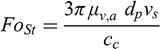
When the Reynolds number is very small (Re ≪ 1), the force, Fo_St, exerted by the fluid (here the air) on a moving particle or droplet may be written as follows:

FoSt=3 π μv,a dpvscc (11.1)

where μ_v,a is the dynamic viscosity of the air (kg m⁻¹ s⁻¹), d_p is the diameter of the particle (or droplet) (m), v_s is the particle sedimentation velocity (m s⁻¹), and c_c is the Cunningham correction factor, which is a function of the particle size. The Cunningham factor is a correction that applies to fine and ultrafine particles (it is equal to 1.01 for a particle with a diameter d_p = 10 μm, 1.16 for d_p = 1 μm, 2.8 for d_p = 0.1 μm, and 22 for d_p = 0.01 μm). This formula applies to ultrafine and fine particles and to some coarse particles, because for particles with a diameter less than 10 μm, Re < 2.5 × 10⁻³.

When the Reynolds number is greater (Re ≫ 1), the following expression applies:

FoSt= π cd ρa dp2 vs28 cc (11.2)

where c_d is the drag factor (or drag coefficient), ρ_a is the air density, and the other terms are the same as in the previous formula. The drag coefficient is a function of Re and, therefore, depends on the particle size since: Re = ρ_a d_p v_s /μ_v,a. This formula applies to very large particles and droplets (d_p > 50 μm), for example raindrops and some dust particles.

The acceleration of a particle (or droplet) moving in the atmosphere is governed by gravity, the buoyant force due to displacement of the fluid (Archimedes’ principle), and the air resistance:

mp dvsdt=mp g−mair g−FoSt(11.3)

The mass of the particle or droplet (m_p) is about 1,000 times greater than that of the displaced air (m_air) and the corresponding buoyant force (m_air g) may, therefore, be neglected. The particle or droplet reaches its terminal fall velocity (dv_s/dt = 0) when the friction due to the air resistance compensates gravity:

Thus, the terminal sedimentation velocity (v_s^f) may be calculated for the two regimes defined in Equations 11.1 and 11.2 for Stokes’ law. If Re ≪ 1 (particles and fog droplets):

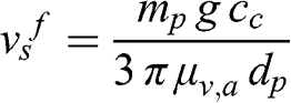vsf=mp g cc3 π μv,a dp(11.5)

The particle mass may be expressed as a function of its diameter and density:

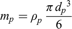mp=ρp π dp36(11.6)

Then, the terminal fall velocity of the particle as a function of its diameter and density is as follows:

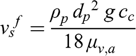vsf=ρp dp2 g cc18 μv,a (11.7)

For an atmospheric particle or fog droplet, the final fall velocity is proportional to the square of its diameter (however, the Cunningham correction modifies this simple relationship); therefore, it decreases as its diameter decreases.

If Re ≫ 1 (large dust particles and raindrops):

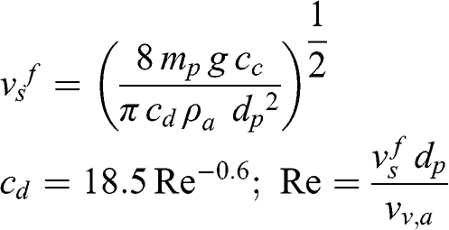vsf=(8 mp g ccπ cd ρa  dp2)12cd=18.5 Re−0.6; Re=vsf dpνv,a(11.8)

where ν_v,a is the kinematic viscosity of the air. Therefore, the terminal fall velocity must be calculated by iteration since it depends on the drag coefficient, which depends via the Reynolds number on the fall velocity. Expressing the mass of a particle or drop as a function of its density and diameter:

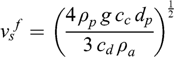vsf=(4 ρp g cc dp3 cd ρa)12(11.9)

Thus, the terminal fall velocity is proportional to the square root of the particle diameter (with a correction due to the drag coefficient). For raindrops, the simplified Kessler formula may be used (Kessler, 1969):

vsf=130 dr(11.10)

where v_s^f is the raindrop fall velocity (m s⁻¹) and d_r is the raindrop diameter (m). The difference between these two equations is <10 % for a raindrop of 1 mm: 4.5 m s⁻¹ with Equation 11.9 and 4.1 m s⁻¹ with Equation 11.10. These formulas tend to overestimate the terminal fall velocity of drops greater than 2.5 mm. More detailed parameterizations are available that better represent the fall velocity of raindrops over a wide range of sizes (see the review by Duhanyan and Roustan, 2011). Note that raindrops rarely have diameters greater than 6 mm, because they tend to break into several smaller drops when they get bigger.

11.1.2 Interception and Inertia

Deposition by interception and inertia concerns atmospheric particles that may interact with surfaces via these processes and then deposit. When the air flow must go around an obstacle, particles present in the air may get into contact with the obstacle either because of their size or mass. The size of a particle is much greater than that of an air molecule and the particle may, therefore, interact with the obstacle because of its size. This interception process is roughly proportional to the cross-section of the particle, i.e., (π d_p²). On the other hand, the mass of a particle leads to inertia when the air flow changes direction to go around an obstacle. This inertia is roughly proportional to the particle mass, i.e., proportional to its volume, (π d_p³/ 6). Therefore, these two processes are negligible for ultrafine particles and are only relevant for fine particles (0.1 μm < d_p < 2.5 μm) and coarse particles (d_p > 2.5 μm).

These processes of impact by inertia and interception are also essential for technologies of particulate matter emission control (see Chapter 2). For example, cyclones use inertia and baghouses use interception and inertia to capture particles. Also, atmospheric particles with a diameter greater than a few microns (μm) are captured efficiently by these processes in the nose and upper airways and, therefore, are not transported deeply into the lungs, unlike fine and ultrafine particles (see Chapter 12).

11.1.3 Diffusion

The diffusion of a gas molecule or particle in the atmosphere toward a surface may be considered to include several steps (Wesely, 1989). For all pollutants (gases and particles), two successive steps bring the pollutant in contact with the surface: (1) turbulent mass transfer in the atmosphere toward the surface and (2) diffusive mass transfer within a very thin layer (on the order of a millimeter) in direct contact with the surface. This latter layer is not affected by atmospheric turbulence and is, therefore, considered to be in a quasi-laminar regime. Mass transfer within that layer occurs by molecular diffusion for gases and via brownian diffusion for particles. In addition, the processes of impact by inertia and interception for particles take place within that layer. Typically, one considers that particles deposit on a surface once they get into contact with that surface (a bouncing coefficient may be used in some cases to account for the fact that some particles may bounce and, therefore, will not remain on the surface). For gases, a third step is included. It determines the deposition rate by absorption into the surface (for example, dissolution into a dew layer), adsorption onto the surface (for example, adsorption onto activated carbon) or chemical reaction at the surface (for example, an acid gas may react with an alkaline surface). A combination of absorption or adsorption followed by chemical reaction may also occur. For particles, inertia and interception processes are important in the case of deposition on surfaces with complex geometries, such as vegetation, for particles with a diameter between about 1 and 10 μm.

This series of processes represents the overall dry deposition phenomenon by diffusion and it may be seen as a series of resistances to mass transfer, by analogy with an electrical circuit.

Aerodynamic Resistance

The first step is associated with an aerodynamic resistance and pertains to the turbulent mass transfer of the pollutant (gas molecule or particle) in the atmosphere toward a layer near the surface. Therefore, it is governed by the vertical transport processes, i.e., vertical atmospheric dispersion. This transfer resistance is large when the atmosphere is stable. It is small when the atmosphere is unstable; then, turbulence readily brings pollutants into contact with the surface via vertical mixing.

The vertical mass flux, F_d, due to this turbulent process may be calculated using a first-order closure of atmospheric turbulence. A K type turbulence representation is generally used (the negative sign is used here because the flux corresponds to a sink for the atmospheric compartment):

Fd=−KzdCdz(11.11)

The vertical dispersion coefficient may be expressed as follows (see Chapter 6):

K_z = κu * z

Kz=κu*z(11.12)

where κ is the von Kármán constant (κ = 0.4) and u_* is the friction velocity. This expression is valid for a neutral atmosphere. If the atmosphere is stable or unstable, the vertical profile of the concentrations in the surface layer differs and this equation must be modified using the parameter Φ_H(z). The corresponding parameter Φ_M(z) for momentum is sometimes used; however, mass transfer is better associated with heat transfer (both are scalars) than with momentum transfer (a vector). Therefore, the temperature profile seems more appropriate for mass transfer than the vertical profile of the horizontal wind speed (see Chapter 4):

Kz=κu*zΦH(z)(11.13)

FdΦH(z) dzκ u*z=−dC(11.14)

Integrating between the reference height (located within the surface layer), z_r, which corresponds to the height of the reference concentration, C, and the bottom of this turbulent layer (taken to be by definition the roughness length, z₀):

Fd∫z0zrΦH(z)κ u*z dz=−∫C0CdC(11.15)

Thus:

Fd=−ΔC∫z0zrΦH(z)  dzκ u*z(11.16)

For a neutral atmosphere (Φ_H(z) = 1):

Fd=−κu*ΔCln(zrz0)(11.17)

The vertical flux may be expressed as a function of the aerodynamic resistance, r_a:

Fd=−ΔCra (11.18)

Thus, r_a may be written as a function of the variables that govern the turbulent mass transfer:

ra=∫z0zrΦH(z) dzκ u*z(11.19)

In the case of a neutral atmosphere, Φ_H(z) = 1, therefore:

ra=ln(zrz0)κ u*(11.20)

In the case of stable or unstable atmospheres, the solution is more complicated, because one must integrate using the profile of Φ_H(z). The profile given in Equation (4.68) is used for a stable atmosphere and the integration leads to the following solution for r_a:

ra=0.95ln(zrz0)+7.8 (zr−z0)LMOκ u*(11.21)

where L_MO is the Monin-Obukhov length (see Chapter 4). The profile given in Equation (4.69) is used for an unstable atmosphere and the integration leads to the following solution:

ra=0.95 κ u*[ln[(1−11.6zrLMO)12−1(1−11.6zrLMO)12+1]−ln[(1−11.6z0LMO)12−1(1−11.6z0LMO)12+1]](11.22)

These formulations imply several assumptions and they apply in theory only within the surface layer, i.e., the layer where the vertical fluxes for momentum, heat, and mass are constant with height. This surface layer ranges from the surface up to a height that varies between a few tens of meters to about 100 m (~10 % of the planetary boundary layer, see Chapter 4).

Resistance Due to Diffusion and Impact Processes

The second step corresponds to a resistance by diffusion in a very thin layer in contact with the surface. This layer (with a thickness on the order of 1 mm) is characterized by a quasi-laminar flow. Therefore, resistance is mostly due to diffusion and is a function of the molecular diffusion coefficient for gases and brownian diffusion coefficient for particles. Molecular diffusion coefficients depend on the physico-chemical properties of the molecule; however, they vary within a rather limited range of values. For example, the diffusion coefficient of carbon monoxide (CO) in the air is 0.12 cm² s⁻¹, that of ozone (O₃) is 0.14 cm² s⁻¹, and that of nitrogen dioxide (NO₂) is also 0.14 cm² s⁻¹.

The resistance to diffusion in the quasi-laminar layer, r_b, is defined as follows:

rb=5 Sc23 u*(11.23)

where u_* is the friction velocity (u*2=−u‘w‘¯ ) and Sc is the Schmidt number, which characterizes the relative importance of advection and diffusion (it corresponds to the Prandtl number, which is used in heat transfer):

Sc=νv,aDm(11.24)

where ν_v,a is the kinematic viscosity of the air (m² s⁻¹; the kinematic viscosity is related to the dynamic viscosity via the fluid density: ν_v,a = μ_v,a / ρ_a) and D_m is the molecular diffusion coefficient of the gaseous pollutant in the air (m² s⁻¹).

For a particle, mass transfer within the quasi-laminar layer depends on brownian diffusion. However, inertia and interception processes also take place within that layer and they are, therefore, treated jointly with diffusion. The following empirical formula may be used (Zhang et al., 2001):

rb=13u*(EB+EIM+EIN) fp(11.25)

where E_B, E_IM, and E_IN are collection efficiencies of brownian diffusion, impact by inertia, and interception, respectively, and f_p is a correction factor representing the fraction of particles that stick to the surface after contact:

EB=Sc−2/315EIM=(Stα+St)βEIN=12(dpdf)2(11.26)

where Sc is defined as in Equation 11.24 for gaseous molecules, but using the brownian diffusion coefficient, D_p, instead of the molecular diffusion coefficient, St is the Stokes number, d_p is the particle diameter, d_f is a characteristic dimension of the surface (vegetation leaf, filter …), and α and β are empirical parameters that depend on the surface type. Zhang et al. (2001) proposed some values for these parameters depending on surface type: α ranges between 0.6 and 100, β = 2, and d_f ranges between 2 and 10 mm. Here, the brownian diffusion term, E_B, has been modified to be consistent with (1) the formulation of the molecular diffusion for gaseous pollutants and (2) the experimental data of Möller and Schumann (1970). The Stokes number is a characteristic of both the particle and the flow; the smaller the particle, the smaller St. It is defined differently for vegetation-covered surfaces and smooth surfaces:

Stvegetation=vs u*g dfStsmooth=vs u*2g νv,a(11.27)

where v_s is the particle sedimentation velocity, u_* is the friction velocity, d_f is the characteristic length of the surface, and ν_v,a is the kinematic viscosity of the air.

The brownian diffusion coefficient of a particle decreases with increasing particle size, whereas the mass transfer velocities for inertia, interception, and sedimentation increase with increasing particle size. As a result, ultrafine particles (i.e., those with a diameter less than 0.1 μm) and coarse particles (i.e., those with a diameter greater than 2.5 μm) have lower resistances than fine particles (i.e., those with a diameter less than 2.5 μm but greater than 0.1 μm), because ultrafine particles are rapidly deposited via brownian diffusion and coarse particles are deposited effectively via sedimentation, inertia, and interception. Figure 11.1 shows the contributions of these different deposition processes as a function of particle diameter. Conditions used in this figure correspond to deposition over grassland under neutral atmospheric conditions with a friction velocity of 0.5 m s⁻¹, a roughness length of 0.01 m, a particle density of 1.5 g cm⁻³, and a characteristic length of 2 mm for grass. Under these conditions, dry deposition via interception is negligible compared to the other processes. The aerodynamic resistance limit is indicated. Note that sedimentation is not affected by the aerodynamic resistance, whereas all other processes are. Therefore, the process of deposition via inertia, which is commensurate with sedimentation up to a particle diameter of about 10 μm, becomes capped for larger particles.

Figure 11.1. Dry deposition velocities of particles as a function of diameter (u_* = 0.5 m s⁻¹, z₀ = 0.01 m, ρ_p = 1.5 g cm⁻³, d_f = 2 mm).

Total Resistance

The total resistance to atmospheric deposition is simply the sum of these two or three resistances. It is expressed in s m⁻¹. The deposition velocity is the inverse of the resistance and it is expressed in m s⁻¹. The vertical mass flux is constant in the surface layer and for gaseous pollutants the following relationships may be written (for particles, the last equation is not taken into account):

Fd=−ΔaCra=−ΔbCrb=−ΔcCrc(11.28)

where the subscript of Δ represents the atmospheric layer of interest for the corresponding resistance. The total resistance is obtained from the overall concentration difference:

Fd=−ΔtCrt(11.29)

Δ_tC = Δ_aC + Δ_bC + Δ_cC

ΔtC=ΔaC+ΔbC+ΔcC(11.30)

Thus, for the overall concentration difference:

Δ_tC = −F(r_a + r_b + r_c)

ΔtC=−F(ra+rb+rc) (11.31)

Therefore:

r_t = r_a + r_b + r_c

rt=ra+rb+rc(11.32)

It may be noted that, in the resistance approach, the atmospheric layer between the roughness height, z₀, and the quasi-laminar layer is not treated, which implies that mass transfer through that layer is not limiting compared to mass transfer in the other layers, i.e., the quasi-laminar layer in the case of unstable atmospheric conditions or the planetary boundary layer in the case of stable conditions.

11.1.4 Dry Deposition Velocities and Fluxes

For particles, sedimentation must be combined with the diffusion, interception, and inertia processes to obtain the full dry deposition process. The correct expression is obtained by combining the deposition fluxes to derive the total deposition velocity, v_d (Venkatram and Pleim, 1999):

vd=vs(1−exp(−rt vs))(11.33)

where v_s is the sedimentation velocity and r_t is the resistance to deposition by diffusion, interception, and inertia (i.e., the inverse of the dry deposition velocity due to these three processes). Thus, as v_s tends toward 0 (ultrafine or fine particle), v_d tends toward (1/r_t); as v_s ≫ 1 / r_t (coarse particle), then, v_d tends toward v_s. Figure 11.1 shows the importance of sedimentation for coarse particles, because it is not limited by the aerodynamic resistance.

The dry deposition velocities differ among pollutants (gaseous molecules and particles of various sizes), atmospheric conditions (which affect turbulence), and surface type (soil, vegetation, buildings, water, …). A chemical species that is highly water soluble, such as nitric acid, may have a dry deposition velocity that is several cm s⁻¹ during daytime (i.e., when atmospheric turbulence is significant). On the other hand, fine particles have deposition velocities that are on the order of 0.1 cm s⁻¹ during daytime. At night, stable atmospheric conditions may reduce deposition velocities by an order of magnitude or more. Generally, dry deposition velocities are greater in forested areas than over grassland, because the available surface area of tree leaves is much greater than the projected ground surface area.

The deposition flux is the mass of pollutant (g) that is deposited per unit surface area (m²) per unit time (s). Therefore, the dry deposition flux is equal to the dry deposition velocity multiplied by the pollutant concentration, taken to be negative as it is a sink term for the atmosphere:

The change with respect to time of the atmospheric concentration of a pollutant that is affected only by dry deposition may be calculated via a mass balance on the atmospheric layer affected by dry deposition. As a first approximation, the planetary boundary layer (PBL), which during daytime is typically a well-mixed layer, may be used to carry out this mass balance. Therefore, given a volume of air of surface area A and height z_i (i.e., the PBL height), the pollutant mass, M, present in that volume is:

The quantity of pollutant that is deposited per unit time is: A F_d = −Av_d CA Fd=−A vd C . Therefore, the change with respect to time of the pollutant concentration is governed by the following ordinary differential equation:

dMdt=A Fd(11.36)

Therefore:

d(C A zi)dt=− A vd C; thus: dCdt=−vdziC(11.37)

The solution is as follows:

C=C0 exp(−vdzit)(11.38)

where C₀ is the initial concentration at t = 0. The term (v_d / z_i) is equivalent to a kinetic constant for a first-order process.

11.2.1 Processes

Wet deposition includes several processes. Generally, a distinction is made between wet deposition associated with precipitation (rain, snow, hail) and occult wet deposition associated with the impact of cloud droplets on elevated terrain (e.g., a mountain) and the sedimentation of fog droplets. Wet deposition by precipitation scavenging dominates and rain scavenging tends to be the most important process, because raindrops can absorb larger amounts of pollutants than snow flakes or ice crystals.

During a precipitation event, two main processes contribute to wet deposition. One process takes place within the cloud, whereas the other process takes place below the cloud base. Within a cloud, during its formation, particles act as condensation nuclei for the formation of cloud droplets (which may later become raindrops) and the pollutants present initially in those particles become incorporated into those droplets. Furthermore, gaseous and particulate pollutants are captured by cloud droplets and raindrops within the cloud. Gaseous pollutants are captured by dissolution in the aqueous phase. Particles are captured when the particle collides with a cloud droplet or raindrop. These processes taking place within the cloud are considered to constitute an overall process called rainout.

Then, precipitation scavenges a fraction of the pollutants present in the atmosphere between the Earth’s surface and the cloud base. This scavenging occurs via dissolution of water-soluble gaseous pollutants and capture of particles via collisions between a particle and a raindrop. This below-cloud scavenging is called washout. Thus, water solubility of a gaseous pollutant increases its scavenging efficiency. For particles, brownian diffusion, interception, and impact by inertia contribute to the precipitation scavenging process to various extents depending on particle size. Brownian diffusion dominates for ultrafine particles, interception tends to be the major process for fine particles between 0.1 and 1 μm, and impact by inertia dominates for the larger particles (typically, those with a diameter greater than 1 μm). In the case of interception, a larger particle has a greater probability to enter into contact with a raindrop than a small particle. In the case of inertia, a light particle is more likely to follow the air flow around a raindrop than a heavy particle, which may then collide with the raindrop. The collection efficiency of particles by raindrops is minimum for fine particles (those with a diameter between 0.1 and 2.5 μm) compared to those of ultrafine particles (diameter less than 0.1 μm) and coarse particles (diameter greater than 2.5 μm). The efficiency of this scavenging may be represented quantitatively by a scavenging coefficient, which can be calculated theoretically or estimated empirically. This scavenging coefficient depends on the water solubility of gaseous pollutants and on the size and density of particles. It depends also on precipitation intensity and on the raindrop size distribution.

11.2.2 Parameterizations

The mass transfer of gaseous and particulate pollutants from the gas phase to cloud droplets or raindrops comprises several processes including the activation of hygroscopic particles, collision of particles with droplets, and diffusion of molecules and gas/liquid equilibrium for gaseous pollutants. The parameterization of these processes is described here. Scavenging of pollutants by snow is less efficient than scavenging by rain and, consequently, the former has been little studied. Therefore, only rain scavenging is presented here.

Parameterization of Washout for Gaseous Pollutants

The dynamic mass transfer of a molecule from the gas phase to the raindrop surface may limit pollutant scavenging because gas/raindrop equilibrium may not be reached. The terminal fall velocity of a raindrop of 5 mm is about 9 m s⁻¹. If the cloud base is at 2,000 m above ground level, the raindrop lifetime is less than four minutes. This time period is commensurate with that mentioned previously for cloud droplets. However, mass transfer of a gas molecule to a cloud droplet with a diameter of a few tens of microns is faster than that of a molecule to a raindrop with a diameter of a few millimeters, as shown in the following equations.

The mass transfer flux, F_m (g m⁻² s⁻¹), of the pollutant from the gas phase to the raindrop is expressed as a function of (1) the concentration gradient between the gas phase and the raindrop surface and (2) a mass transfer coefficient:

F_m = k_m(C_g − C_g,e)

Fm=km(Cg−Cg,e)(11.39)

where k_m is the mass transfer coefficient (m s⁻¹), C_g is the bulk gas-phase concentration, and C_g,e is the gas-phase concentration at the surface of the drop (i.e., in thermodynamic equilibrium with the aqueous-phase concentration according to Henry’s law). These concentrations are expressed here in g m⁻³. The mass transfer coefficient may be written as a function of dimensionless numbers:

km=ShDmdr(11.40)

where Sh is the Sherwood number (which characterizes the ratio of total mass transfer and transfer by diffusion), D_m is the molecular diffusion coefficient of the gaseous pollutant in the air (m² s⁻¹), and d_r is the raindrop diameter (m). The Sherwood number is related to the Reynolds number, which characterizes the flow as the ratio of advection (or convection) and viscosity, and the Schmidt number, which characterizes the ratio of viscosity and diffusion:

Sh = 2 + 0.6 Re^1/2 Sc^1/3

Sh=2+0.6 Re1/2 Sc1/3(11.41)

where Re and Sc were defined in Section 11.1. Therefore:

km=Dmdr(2+0.6 (vs,r dr)1/2(ρaμv,a)1/6Dm−1/3)(11.42)

where v_s,r is the fall velocity of the raindrop (m s⁻¹). The mass transfer coefficient, k_m, is inversely proportional to the raindrop diameter when the raindrop fall velocity is low or to the square root of the raindrop diameter when the raindrop fall velocity is high. In any case, mass transfer is slower for a larger raindrop.

A mass balance on a raindrop leads to the following equation:

dMaqdt=Fm sr(11.43)

where M_aq is the pollutant mass in the raindrop (i.e., in the aqueous phase, in g), which changes as a function of the mass transferred from the gas phase to the raindrop, and s_r is the surface of the raindrop (m²). Therefore, this mass transfer rate is proportional to the mass transfer flux, F_m, and the raindrop surface area. The pollutant mass in the raindrop may be expressed as a function of the pollutant concentration in the raindrop and the raindrop volume:

M_aq = C_aq v_r

Maq=Caq vr(11.44)

where C_aq is the concentration of the pollutant in the raindrop (g m⁻³) and v_r is the raindrop volume (m³). By definition:

vr=π dr36; sr=π dr2(11.45)

In addition, the aqueous-phase concentration is related to the gas-phase concentration at the raindrop surface by Henry’s law (using the standard Henry’s law constant or the effective Henry’s law constant depending on the pollutant, expressed in M atm⁻¹):

C_aq = H(C_g,e RT) × 10³

Caq=H (Cg,e R T)×103 (11.46)

where R is the ideal gas law constant (atm m³ mole⁻¹ K⁻¹), T is the temperature (K) and the factor 10³ is used to convert the volume from liters to m³. If the atmosphere below the cloud base is significantly polluted compared to the air where the cloud is located (for example, if the cloud base is above the PBL), then C_g ≫ C_g,e, and the mass transfer flux may be simplified as follows: F_m = k_m C_g. Thus:

dCaqdt=6 km Cgdr(11.47)

Assuming that the atmosphere below the cloud base is well mixed (C_g = constant):

Caq=6 km Cgdrt(11.48)

where t corresponds here to the lifetime of the raindrop. It is assumed here that C_aq(t = 0) = 0. The raindrop lifetime depends on the raindrop fall velocity, v_s,r : t = h_c / v_s,r, where h_c is the height of the cloud base above ground level:

Caq=6 km Cg hcdr vs,r  (11.49)

It is assumed here that the raindrop does not become saturated with the pollutant. The wet deposition flux, F_w, is the quantity of pollutant deposited per unit surface area per unit time. It corresponds to the product of the pollutant concentration in the raindrops, C_aq, and the precipitation intensity (m of precipitation per second), I_p (a negative sign is used here to treat the wet deposition flux as an atmospheric sink):

F_w = −C_aq I_p

Fw=−Caq Ip(11.50)

Therefore:

Fw=−6 km Cg hc Ipdr vs,r(11.51)

The scavenging coefficient, Λ(s⁻¹), is defined as the kinetic constant corresponding to the loss of air pollutant via wet deposition in the air column below the cloud base:

dCgdt=−Λ t(11.52)

Therefore:

C_g(t) = C_g0 exp(−Λ t)

Cg(t)=Cg0exp(−Λ t)(11.53)

where C_g0 is the pollutant concentration at the beginning of the precipitation event. A mass balance on an air volume of surface area A and height h_c (from the surface to the cloud base, i.e., the air volume scavenged by rain) leads to the mass of pollutant, M, available for scavenging by precipitation:

M = C_gAh_c = C_g0 exp(−Λt)Ah_c

M=Cg Ahc=Cg0exp(−Λt) Ahc(11.54)

The wet deposition flux for a time period dt is the quantity of pollutant scavenged per unit surface area and per unit time. Therefore, deriving Equation 11.54 with respect to t:

Fw=1AdMdt=−Cg(t) Λ hc(11.55)

Reconciling the two formulations for F_w, Equations 11.51 and 11.55, the scavenging coefficient may be written as a function of the precipitation intensity, mass transfer coefficient, raindrop diameter, and raindrop fall velocity:

Λ=6 km Ipdr vs,r(11.56)

The scavenging coefficient appears to be proportional to the precipitation intensity. However, a more intense precipitation tends to involve larger raindrops, which have greater fall velocities. Therefore, the scavenging coefficient is not proportional to precipitation intensity. For example, the scavenging coefficient of nitric acid is estimated to be 5 × 10⁻⁵ s⁻¹ for a precipitation intensity of 1 mm h⁻¹, whereas it is estimated to be only 2 × 10⁻⁴ s⁻¹ (i.e., four times greater) for a precipitation intensity of 10 mm h⁻¹ (i.e., ten times greater).

Parameterization of Particle Scavenging

Particle scavenging results from the collision of raindrops with particles and the incorporation of the particle within the raindrop. It is generally assumed that the incorporation process is 100 % efficient.

The collision rate between a raindrop and a particle is proportional to the cross-section area of both the particle and raindrop and to the difference between their fall velocities, v_s,r and v_s,p:

Λ=π4(dr+dp)2 (vs,r−vs,p) E(dr, dp)Nrp(11.57)

where the subscripts r and p refer to raindrop and aerosol particle, respectively, E(d_r, d_p) is the collision efficiency resulting from the diffusion, interception, and inertia processes, and N_rp is the number concentration of raindrops for that precipitation event. In these collision processes, the raindrop plays the role of the surface in the formulations presented in Section 11.1 for dry deposition. This collision rate is equivalent to the scavenging rate if each collision results in the incorporation of the particle within the raindrop. The following formulation (Slinn, 1983) may be used to represent the collision processes between a raindrop and an atmospheric particle. These processes include brownian diffusion, interception, and impact by inertia:

E(dr, dp)=4Re Sc(1+0.4 Re1/2 Sc1/3+0.16 Re1/2 Sc1/2)              +4dpdr(μν,wμν,a+(1+2 Re1/2)dpdr)+(1−0.9 St1/2)(ρpρw)1/2(11.58)

where Re is the Reynolds number of the air flow around the raindrop (defined in Equation 11.8), μ_v is the dynamic viscosity, ρ is the density, the subscript a refers to air, and the subscript w refers to water. The first term on the right-hand side represents the collision of particles with raindrops due to brownian motion of particles. The second term represents the interception process. The third term represents collision by inertia. Here, the simplification of Jung et al. (2003) is used for the inertia term. Figure 11.2 shows the collision efficiency for monodispersed precipitation (i.e., with a single raindrop size) of various intensities. It appears that the collision efficiency is minimum for fine particles, i.e., those particles of diameter between 0.1 and 2.5 μm. This range is called the Greenfield gap , after Stanley Greenfield (1957) of Rand Corporation, who first identified experimentally this minimum in the scavenging efficiency of atmospheric particles by rain.

Figure 11.2. Scavenging of particles by raindrops. Top figure: collision efficiency of particles by raindrops with a diameter of 1.37 mm and a rain intensity of 5 mm h⁻¹, as a function of particle diameter; bottom figure: scavenging coefficient for several rain intensities as a function of particle diameter.

For a strong precipitation intensity, the following assumptions may be introduced: d_r ≫ d_p; v_s,r ≫ v_s,p. Then:

Λ=π4  dr 2  vs,r E(dr,dp) Nrp(11.59)

The precipitation intensity may be expressed by conducting a mass balance on the rain water (i.e., the volume of all raindrops per volume of air multiplied by the raindrop fall velocity). For a monodispersed rain:

Ip=π6  dr3  vs,r Nrp(11.60)

Therefore, the scavenging coefficient may be written as a function of the precipitation intensity, the scavenging efficiency, and the raindrop diameter:

Λ=32  IpE(dr,dp) dr(11.61)

Several formulations are available to represent the relationship between the rain intensity and the raindrop size distribution (e.g., Duhanian and Roustan, 2011). For the sake of simplicity, a monodispersed precipitation may be used with a simple relationship between the rain intensity and the mean raindrop diameter: d_r = 0.976 I_p^0.21, where I_p is in mm h⁻¹ and d_r is in mm (Pruppacher and Klett, 1998). Figure 11.2 shows the raindrop/particle collision efficiency and the scavenging coefficient as a function of the particle diameter for different raindrop diameters and rain intensities. The scavenging rate is a function of the rain intensity. However, it is inversely proportional to the raindrop diameter (which increases with the rain intensity) and proportional to the collision efficiency (which is a complicated function of the raindrop and particle diameters). For example, the scavenging coefficient of a particle with a diameter of 2.5 μm is 3.7 × 10⁻⁷ s⁻¹ for a rain intensity of 1 mm h⁻¹ and it is 2.1 × 10⁻⁶ s⁻¹ (i.e., seven times greater) for a rain intensity of 25 mm h⁻¹ (i.e., 25 times greater).

Example: Calculation of the fraction of nitric acid that is removed from the atmosphere via wet deposition

It is assumed that the rain event lasts one hour and that the scavenging coefficient of nitric acid (HNO₃) is 1.5 × 10⁻⁴ s⁻¹. It is assumed that there is no nitric acid within the cloud and that nitric acid is uniformly mixed within a PBL of 2,000 m.

The change with respect to time of the nitric acid concentration in the PBL due to rain scavenging is given by Equation 11.53:

[HNO₃(g)](t) = [HNO₃(g)]₀ exp(−Λt)

[HNO3(g)](t)=[HNO3(g)]0 exp(−Λ t)

Therefore, after one hour (3,600 s):

[HNO3(g)](t=1 h)[HNO3(g)]0=0.58

Therefore, 58 % of the initial nitric acid remain in the atmosphere and 42 % have been removed by rain. The amount of nitric acid scavenged by rain in one hour is commensurate with that deposited via dry processes in 12 hours. Note that the PBL height does not come into play in the calculation because scavenging affects the entire column below the cloud base.

11.3.1 General Considerations

Some pollutants that have been deposited on surfaces may be reemitted into the atmosphere. It is important to take these reemission processes into account in order to (1) develop complete emission inventories of air pollution and (2) develop a better understanding for some pollutants of the net balance of their mass transfer between the atmosphere and some ecosystems.

This reemission process may occur in different ways. In its simplest form, the pollutant is reemitted under the same form as it was deposited. Semi-volatile pollutants such as persistent organic pollutants (POP) have a volatility that varies with temperature. They deposit more readily when the temperature is low as they are mostly present in the particulate phase. When the ambient temperature increases, their gas/particle partitioning tends to shift toward the gas phase and they are reemitted as gases. A succession of deposition and reemission steps of a semi-volatile pollutant is called the “grasshopper effect,” because the pollutant may be transported over long distances (several thousands of kilometers) via a series of deposition/reemission “hops.”

The reemission of a pollutant may also occur following a chemical transformation. This is the case, for example, for the emission of some nitrogen oxides (NO and N₂O) from soils following denitrification of nitrate compounds. This is also the case for mercury, which may deposit as gaseous oxidized mercury (for example, as mercury chloride, which is highly water soluble) and, following reduction in soil or surface waters, it may be reemitted as elementary mercury, which is little water soluble and very volatile.

Particles that have been deposited may be reemitted either because of wind-related processes (aeolian resuspension) or because of anthropogenic activities (agricultural activities, on-road traffic …). Also, particles may be emitted naturally into the atmosphere via aeolian erosion (e.g., from highly erodible soils, such as deserts) and via the evaporation of droplets from waves leading to the emission of sea salt particles into the atmosphere.

Currently, the processes leading to the reemission of gases and particles and to the natural emissions of particles from surfaces are poorly characterized and there are significant associated uncertainties. Three major processes of reemissions and natural emissions of particles are described in the following sections: (1) the resuspension of particles by on-road traffic, (2) the natural emission of particles from soils via aeolian erosion, and (3) the natural emission of sea salt particles.

11.3.2 Resuspension of Particles by On-road Traffic

Empirical estimates and numerical modeling suggest that the resuspension of particles by on-road traffic may contribute significantly to ambient PM₁₀ concentrations in the vicinity of major roadways. Therefore, it is essential to account for this particle resuspension term in PM emission inventories, especially for urban areas. Although the size distribution of resuspended particles suggests that they are mostly large particles, the coarse fraction with diameters between 2.5 and 10 μm may contribute significantly to ambient PM₁₀ concentrations. This resuspension process depends on several factors including the types of vehicles (a heavy-duty vehicle will lead to greater amounts of particle resuspension than a passenger vehicle), the vehicle speed, the traffic flow, and the erodibility of the particles present on the roadway. This erodibility is closely related to humidity, because a dry roadway is more conducive to particle resuspension than a wet roadway. In addition, the amount of particles potentially available for resuspension is an important factor. Several empirical, semi-empirical, and process-based models have been developed to simulate quantitatively the resuspension rate of particles by on-road traffic. The Nortrip model developed by Denby et al. (2013) appears to be the most complete model, because it takes into account all the relevant factors. In particular, Nortrip uses a mass balance to estimate the quantity of particles present on the roadway and potentially available for resuspension. The change with respect to time of the mass of particles per unit length present on the roadway, M_l,r (g km⁻¹), is calculated as follows:

dMl,rdt=Fl,r−Sl,r(11.62)

where t is time (h), F_l,r represents the addition of particles onto the roadway, and S_l,r represents the loss (sink) of particles from the roadway (g km⁻¹ h⁻¹). The addition of particles includes processes that are directly related to on-road traffic, such as brake wear, tire wear, and road wear. These wear processes lead to the emission of particles into the atmosphere, but also to the formation of coarse particles that may deposit immediately on the roadway rather than being emitted to the atmosphere. The addition of particles may also include activities such as sanding and salting of roadways during snow episodes. Finally, atmospheric deposition of particles (see Section 11.1) could contribute to the addition of particles to roadways, although the small dry deposition velocities of atmospheric particles suggest that the direct contribution of traffic-related processes should dominate. The loss terms include mostly the resuspension of particles by traffic and the removal of particles during rain events via water runoff.

Taking into account only the addition of particles due to traffic:

Fl,r=∑v=12Nv∑w=13Wv,w(11.63)

where the subscript v represents the vehicle type (here, heavy-duty vehicles and light-duty vehicles, including passenger cars) and the subscript w represents the wear processes for brakes, tires, and road surface, N_v is the number of vehicles per hour (traffic flow), and W_v,w is the wear rate in g of particles per vehicle per km. The wear rates for tires and road surface are expressed as a function of vehicle speed. The brake wear rate depends on the type of driving (road, urban, congested traffic …). Denby et al. (2013) provide data to calculate those wear rates.

The loss term corresponding to particle resuspension may be written as follows:

Sl,r=Ml,r∑v=12Nvfv(vv)(11.64)

where f_v is the particle mass fraction present on the roadway that is resuspended by a vehicle. This fraction depends on the vehicle type (subscript v) and its speed, v_v. Denby et al. suggest using f_v,ref = 5 × 10⁻⁶ per vehicle for light-duty vehicles (including passenger cars) and f_v,ref = 5 × 10⁻⁵ per vehicle for heavy-duty vehicles at a reference speed of 70 km h⁻¹. A loss term may also be calculated for particle removal during rain events; however, this calculation requires detailed information on the rain event (duration and rain intensity). As a first approximation, the particle mass present on the roadway can be reset to zero after each significant rain event.

The equation of change of the particle mass present on the roadway may be written as follows for dry periods between rain events:

dMl,rdt=Fl,r−Ml,r∑v=12Nvfv,refvvvv,ref(11.65)

where the subscript ref corresponds to values at the reference speed and particle resuspension is assumed to be proportional to vehicle speed. At steady state, assuming M_l,r(t=0) = 0:

Ml,r(t)=Fl,r∑v=12Nvfv,refvvvv,ref(1−exp(−∑v=12Nvfv,refvvvv,ref t))(11.66)

The particle resuspension emission rate by on-road traffic is obtained by combining Equations 11.63 and 11.66. Figure 11.3 shows the resuspension rates for an urban freeway and a suburban boulevard in France. They are compared to the direct particulate emissions due to exhaust and wear processes (brakes, tires, and road surface) (Thouron et al., 2018). Direct emissions were calculated using the Copert 4 emission factors (see Chapter 2). These two roadways have very different characteristics. The urban freeway in the Grenoble region in southeastern France has an average traffic flow of 4,000 vehicles per hour with 4 % of heavy-duty vehicles and an average traffic speed of 69 km h⁻¹. The suburban boulevard in the Paris region has an average traffic flow of 800 vehicles per hour with 3 % of heavy-duty vehicles and an average traffic speed of 32 km h⁻¹. In addition, precipitation was negligible during the Grenoble case study, whereas there were several rain events during the suburban Paris case study. The results show that the contribution of resuspension by traffic to PM₁₀ emissions is much greater for the urban freeway than for the suburban boulevard, because of greater traffic flow, greater traffic speed, and less precipitation (i.e., a dryer roadway). Under these conditions, resuspension is commensurate with direct emissions from traffic for this urban freeway. On the other hand, lower traffic flow and speed, as well as frequent rain events, in the suburban Paris case study lead to a contribution of resuspension by traffic, which is only about 10 % of direct PM₁₀ emissions.

Figure 11.3. PM₁₀ direct emission rates and traffic-related resuspension emission rates. Top figure: An urban freeway near Grenoble, France; bottom figure: a suburban boulevard in the Paris region.

Source: Adapted from Thouron et al. (2018).

The formulas presented previously in this section may be refined to take into account tire types (for example, studded snow tires) and the effect of ambient humidity on the resuspension rate. In addition, the size distribution of resuspended particles must be estimated as a function of the processes involved and, in the case of road wear, traffic speed. Denby et al. (2013) provide parameterizations to estimate particle size distributions.

11.3.3 Particle Resuspension by Wind Erosion

Resuspension of particles from an erodible surface by wind erosion (aeolian resuspension) may contribute significantly to atmospheric particle concentrations and these particles may be transported over long distances (Knippertz and Stuut, 2014). For example, wind erosion episodes in the Sahara desert or the Gobi desert may lead to large ambient PM concentrations in Europe or in Asia, respectively. The aeolian resuspension process consists first of a hydrodynamic lifting of particles available at the surface. When the air flow encounters an obstacle, an acceleration of the flow occurs near the obstacle, which induces a pressure drop. This pressure drop leads to a lift of some of the particles potentially available at the surface. These particles may subsequently deposit back to the surface, especially if they are large particles: this is known as the saltation process. This saltation corresponds to a horizontal particle flux and leads to impacts of particles on the surface. These impacts may fragment the surface and generate particles, which become available for resuspension. Then, a vertical flux of particle resuspension occurs. Models that simulate this vertical flux of particle aeolian resuspension must represent the generation of particles by impact of larger particles via saltation.

A review of the theory and experimental data obtained in wind tunnels and in field programs led to the following expression for the vertical flux of particles resuspended by wind erosion, F_e (Kok et al., 2014):

Fe=ce fer fclay ρa (u*s2−u*t2)u*st (u*su*t)2.7u*st−u*st,refu*st,reffor u*s> u*twith ce=4.4 ×10−5 exp(−2u*st−u*st,refu*st,ref)(11.67)

where c_e is the dimensionless coefficient for the resuspension of particles via wind erosion, f_er is the erodible fraction of the soil surface, f_clay is the clay fraction of the surface (clay content), which corresponds to particles of diameter less than 2 μm (i.e., once resuspended by wind erosion, fine particles), ρ_a is the air density, u_*s is the surface friction velocity, u_*t is the threshold surface friction velocity above which wind erosion occurs, u_*st is the threshold surface friction velocity at standard conditions (here for an air density at 1 atm and 15 °C, i.e., ρ_a = 1.225 kg m⁻³), and u_*st,ref is the reference value of the standard threshold surface friction velocity (i.e., for a surface with optimal erodibility). The threshold friction velocities depend on the nature of the erodible surface and may be measured experimentally. They generally vary between 0.2 and 1.5 m s⁻¹. Thus, the vertical resuspension flux depends on the surface friction velocity, which varies according to the air flow and the surface roughness, and on the nature of the erodible surface, which defines the threshold friction velocity leading to erodibility.

The surface friction velocity corresponds to the component of the friction velocity (see Chapter 4) that pertains to the erodible soil fraction. The surface friction velocity may be calculated from data on surface type (roughness length, size distribution of roughness elements). Okin (2008) proposed an exponential formulation to estimate u_*s from u_* and the height of non-erodible elements, h_ne (for example, vegetation). Measurements suggest that, just downwind of the non-erodible elements, the friction velocity of the surface is 32 % of the friction velocity and that farther downwind the surface friction velocity tends asymptotically toward the friction velocity (being about 90 % of its value at a downwind distance of 10 h_ne). Therefore:

u*s=u*(1−0.68 exp(−x4.8 hne))(11.68)

where x is the distance downwind of the non-erodible element.

An upper limit of the resuspension vertical flux may be estimated for fine particles (u_*st = u_*st,ref):

Fe=4.4×10−5 fer fclay ρa (u*2−u*t2)u*st (11.69)

The comparison of the model of particle resuspension by wind erosion with measurements obtained from field experiments leads to better agreement than earlier models for a range of measured resuspension fluxes spanning more than two orders of magnitude (from 10 to 2,000 μg m⁻² s⁻¹). Most of the calculated fluxes are within a factor of 5 of the measurements and half of the fluxes are within a factor of 2. The uncertainty associated with this model may reach an order of magnitude; however, one should note that the uncertainty associated with the measurements is typically a factor of two. This formulation does not provide any information on the size distribution of the resuspended particles. Particle size distributions for resuspension by wind erosion are available in the scientific literature.

11.3.4 Emissions of Sea Salt Particles

Sea and ocean waves lead to the formation of sea salt droplets in suspension in the air. The evaporation of those droplets may lead to the formation of sea salt aerosol particles. Wave formation depends strongly on wind speed. Different processes are involved in the formation of sea salt droplets. The bursting of bubbles leads to the formation of fine particles (d_p < 1 μm) originating from the bubble surface. The airflow that follows the vacuum generated by the bursting of a bubble leads to the production of larger particles (on the order of 1 to 10 μm). Finally, the separation of the foam from the wave crest leads to coarse particles (>10 μm); this latter process only occurs for very high wind speeds. Therefore, a wide spectrum of sea salt particles results from these various processes. Sea salt particle formation may be important and may affect PM concentrations in coastal areas. Accordingly, several algorithms have been developed to simulate sea salt particle emissions. Monahan et al. (1986) have developed one of the first algorithms that have been widely used to simulate sea salt particle formation. The emission flux may be written as the distribution of the particle vertical flux emitted from the sea surface, F_s, as a function of particle diameter:

dFsddp=function(u10, dp, Tss, ss)(11.70)

This function depends on the wind speed at 10 m, u₁₀, the sea salt aerosol particle diameter, d_p, the sea surface temperature, T_ss (also known as SST for sea surface temperature), and in some cases the sea salinity, s_s. Traditionally, the sea salt particle size is represented by the particle radius at 80 % relative humidity. Since this radius is about twice that of the dry particle, it can be replaced by the dry particle diameter. Grythe et al. (2014) compared about twenty formulations for quantifying sea salt particle emissions. They concluded that the global spatio-temporal variability of sea salt particle emissions was best represented when the emission rate depends not only on wind speed, but also on sea surface temperature.

The influence of the wind speed on sea salt particle emissions is intuitive, since a high wind speed generates greater waves. Typically, functions such as u^α*uα* are used, with α_* ranging between 2 and 3.5 depending on the formulation. However, a conceptual representation of wave formation should use the shear stress of the turbulent airflow, τ_*, rather than the average wind speed at 10 m:

τ*=u*2 ρa(11.71)

where u_* is the friction velocity and ρ_a is the air density. The friction velocity is related to the wind speed via the following equation under neutral conditions (see Chapter 4):

u*=κ u(z)ln(zz0)(11.72)

where κ is the von Kármán constant (κ = 0.4) and z₀ is the roughness length. Therefore, the formation of sea salt particles would be proportional to (τ*)α*/2 .

Laboratory experiments have shown that the emission of sea salt particles depends on temperature. Therefore, taking into account the sea surface temperature is important in order to correctly represent sea salt emissions, for example in the tropics. The physical explanation of this temperature dependence is not obvious. Jaeglé et al. (2011) proposed several explanations. First, the terminal vertical velocity of a bubble is proportional to the kinematic viscosity of sea water and this viscosity depends on temperature. Thus, more bubbles reaching the sea surface lead to more sea salt particle emissions. Second, temperature could affect the mass transfer between bubbles and the surrounding water, which would influence the size distribution of those bubbles reaching the sea surface and, consequently, particle formation. The dependence of coarse mode sea salt particle concentrations on sea surface temperature was approximated by Jaeglé et al. (2011) using a third-order polynomial, thereby leading to the following formula for the sea salt particle emission flux (expressed as a particle-size distributed flux):

dFsddp=(0.3+0.1 Tss,C−0.0076 Tss,C2+0.00021 Tss,C3)×1.373 u103.41 dp−A (1+0.057dp3.45)×101.607 exp(−B2)(11.73)

where

A=4.7(1+30 dp)−0.017dp−1.44B=1−2.3log10(dp)

T_ss,C is the sea surface temperature in °C (T_ss,c = T_ss – 273) and the temperature-dependent term is equal to 1 at T_ss,C ≈ 21°C.