Abstract
This chapter discusses how to apply copulas in water quality analysis. For monthly water quality observations, applications will include (i) a copula-based Markov process to study the water quality sequence with temporal dependence; and (ii) a copula-based multivariate water quality time series analysis. This chapter is in line with Chapter 9.
12.1 Case-Study Sites
According to the availability of water quality data, two watersheds are used as a case study. One watershed is a natural watershed, while the other is an urban watershed. The watershed boundaries and streams data were retrieved from the NHDPlus High Resolution National Hydrography Dataset and Watershed Boundary Dataset (https://nhd.usgs.gov/). The land use and land cover (LULC) were retrieved from the National Land Cover Database (www.nrlc.gov).
12.1.1 Snohomish River Watershed
According to the Department of Ecology of the State of Washington (ecy.wa.gov), the Snohomish River is formed near the city of Monroe, where the Skykomish and Snohomish rivers meet. The Snohomish River continues its way through the estuary of the city of Snohomish before entering into Puget Sound. The Snohomish watershed covers an area of 1,978 square miles (about 5,123 square kilometers) and provides important water recreation activities. In the past, agriculture and forest were two main LULC within the watershed; however, throughout the last century, more human activity has been introduced into the watershed. The Department of Ecology clearly stated (ecy.wa.gov): “over the last century, diking and other engineering activities in the lower part of the basin greatly changed how water is stored and managed in floodplain areas. More recently, cities and suburban areas have grown rapidly, creating more change to the natural water cycle.”
Besides the change in the natural water cycle induced by human activities, water quality issues (including but not limited to bacteria, dissolved oxygen (DO), temperature, and pH) have also been identified for some areas. Four stations located in the Snohomish watershed are selected for the case study: A90, C70, D50, and D130 (shown in Figure 12.1). The total persulfate nitrogen (TPN) and DO at C70 are chosen as the targeting water quality parameters for the temporal dependence case study. DO at all four stations is chosen for the spatial dependence study.
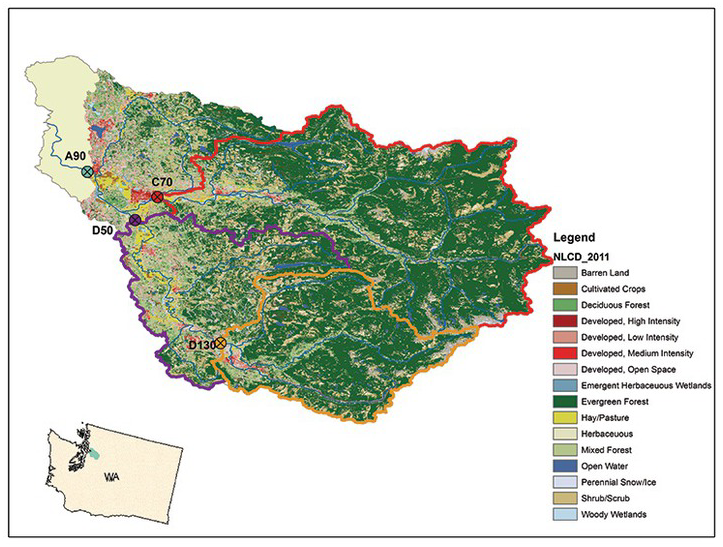
Figure 12.1 Snohomish watershed map and its LULC in 2011(retrieved from USGS and NLCD).
12.1.2 Chattahoochee River Watershed
As a tributary of Apalachicola River, the Chattahoochee River originates south of the Alabama and Georgia border and joins the Apalachicola River at the Georgia and Florida border. The Chattahoochee River watershed is the largest subwatershed of Apalachicola–Chattahoochee–Flint river basin.
The city of Atlanta is located within the watershed. There are gauging stations upstream and downstream of metropolis, i.e., the Belton Bridge station (USGS02332017, upstream) and Whitesburg station (USGS02338000, downstream). The subwatershed upstream of the Bridge station may be classified as the forest watershed. With the major metropolitan area – the city of Atlanta – the subwatershed upstream of Whitesburg is more developed (by 2011, the developed land alone accounts for about 34%) and may be considered the urban watershed (shown in Figure 12.2). The targeting water quality parameters are total nitrogen (TKN, mg/L), DO, and phosphorus (mg/L).

Figure 12.2 Chattahoochee River watershed upstream of the Whitesburg station and its LULC in 2011 (retrieved from USGS and NLCD).
12.2 Dependence Study at the Snohomish River Watershed
In this section, we will investigate the temporal and spatial–temporal dependence for the water quality parameters at the case-study site of the Snohomish River watershed. For the case study of the Snohomish River watershed, monthly TPN (C70 only) and DO (C70, D50, D130, and A90) are applied for the study. The monthly TPN and DO at station C70 are used for the study of temporal dependence. The monthly DO at all four of these stations is applied to study the spatial–temporal dependence.
12.2.1 Study of Temporal Dependence Using Copulas
Temporal Dependence of Monthly TPN and DO at Station C70
The TPN and DO at station C70 are chosen for the study of temporal dependence. Table 12.1 lists the dataset for both temporal and spatial dependence study. We will use the water quality data before 2012 to build a copula-based Markov process model, and the water quality data of 2012 and 2013 will be used for model validation purpose.
Table 12.1. TPN and DO monthly dataset from the Snohomish River watershed.
| Dates | TPN (C70) | DO (C70) | DO (D50) | DO (D130) | DO (A90) |
|---|---|---|---|---|---|
| Oct-94 | 0.116 | 11.3 | 10.8 | 10.5 | 10.9 |
| Nov-94 | 0.312 | 12 | 11.7 | 11.9 | 11.9 |
| Dec-94 | 0.287 | 12.7 | 12.6 | 12.6 | 12.6 |
| Jan-95 | 0.285 | 12.8 | 11.9 | 12.3 | 12.15 |
| Feb-95 | 0.21 | 12.4 | 12.4 | 12.8 | 12.8 |
| Mar-95 | 0.212 | 12.1 | 11.6 | 11.8 | 11.7 |
| Apr-95 | 0.141 | 12.2 | 11.4 | 11.9 | 11.6 |
| May-95 | 0.081 | 11.6 | 10.4 | 11.1 | 10.8 |
| Jun-95 | 0.086 | 11.2 | 10.2 | 10.9 | 10.6 |
| Jul-95 | 0.066 | 10.2 | 9.2 | 9.4 | 9.7 |
| Aug-95 | 0.117 | 10.5 | 9.6 | 9.8 | 9.8 |
| Sep-95 | 0.125 | 10.3 | 9.6 | 9.3 | 9 |
| Oct-95 | 0.253 | 11 | 10.4 | 10.8 | 10.6 |
| Nov-95 | 0.178 | 12.2 | 10.9 | 12 | 11.5 |
| Dec-95 | 0.203 | 12.5 | 11.4 | 12.1 | 11.8 |
| Jan-96 | 0.223 | 12.8 | 11.9 | 12.4 | 12.3 |
| Feb-96 | 0.155 | 12.4 | 12.3 | 12.2 | 12.2 |
| Mar-96 | 0.119 | 12.6 | 11.7 | 12.2 | 12 |
| Apr-96 | 0.114 | 11.7 | 10.8 | 11.3 | 11.1 |
| May-96 | 0.09 | 12 | 11.3 | 11.7 | 11.6 |
| Jun-96 | 0.043 | 11.3 | 10.1 | 10.8 | 10.7 |
| Jul-96 | 0.045 | 10.5 | 9.7 | 9.7 | 10 |
| Aug-96 | 0.107 | 10.1 | 9.4 | 9.6 | 9.8 |
| Sep-96 | 0.194 | 10.7 | 9.9 | 10.5 | 10.2 |
| Oct-96 | 0.331 | 11.6 | 11.4 | 11.7 | 11.3 |
| Nov-96 | 0.237 | 12.3 | 11.8 | 12.2 | 12 |
| Dec-96 | 0.286 | 12.7 | 12 | 12.5 | 12.2 |
| Jan-97 | 0.201 | 13 | 12.3 | 12.6 | 12.4 |
| Feb-97 | 0.232 | 12.5 | 12 | 12.3 | 12 |
| Mar-97 | 0.299 | 12.5 | 11.9 | 12.3 | 12.2 |
| Apr-97 | 0.218 | 12.7 | 12.7 | 12.5 | 12.6 |
| May-97 | 0.077 | 11.9 | 10.9 | 11.8 | 11.2 |
| Jun-97 | 0.076 | 11.6 | 10.8 | 11.2 | 11.1 |
| Jul-97 | 0.058 | 10.2 | 9 | 9.3 | 9.3 |
| Aug-97 | 0.055 | 10.2 | 9.3 | 9.4 | 9.2 |
| Sep-97 | 0.204 | 10.4 | 9.9 | 10.3 | 10 |
| Oct-97 | 0.163 | 11.1 | 10.7 | 11 | 11 |
| Nov-97 | 0.187 | 11.8 | 11.3 | 11.3 | 11.4 |
| Dec-97 | 0.282 | 12.6 | 11.7 | 11.6 | 11.8 |
| Jan-98 | 0.387 | 12.2 | 11.6 | 11 | 11.7 |
| Feb-98 | 0.258 | 12.4 | 11.5 | 11.7 | 11.8 |
| Mar-98 | 0.217 | 12.1 | 11.5 | 12.2 | 11.8 |
| Apr-98 | 0.165 | 12 | 10.9 | 11.5 | 11.5 |
| May-98 | 0.14 | 12 | 11.1 | 11.9 | 11.4 |
| Jun-98 | 0.065 | 10.8 | 9.7 | 10.3 | 10.1 |
| Jul-98 | 0.077 | 10.4 | 9 | 9.9 | 9.3 |
| Aug-98 | 0.075 | 10.1 | 8.3 | 9.4 | 9.1 |
| Sep-98 | 0.097 | 10.3 | 9.6 | 9.4 | 9.4 |
| Oct-98 | 0.23 | 12.1 | 11.7 | 11.5 | 11.2 |
| Nov-98 | 0.378 | 11.7 | 11.2 | 11.5 | 11.4 |
| Dec-98 | 0.392 | 12.6 | 12.4 | 12.6 | 12.2 |
| Jan-99 | 0.333 | 12.2 | 11.9 | 12.1 | 12 |
| Feb-99 | 0.275 | 12.8 | 11.6 | 12.4 | 12.4 |
| Mar-99 | 0.19 | 12.3 | 12 | 12.5 | 12 |
| Apr-99 | 0.162 | 12.4 | 12.1 | 12.7 | 11.9 |
| May-99 | 0.146 | 12.2 | 10.9 | 12.2 | 11.5 |
| Jun-99 | 0.064 | 11.5 | 11.1 | 11.5 | 11.5 |
| Jul-99 | 0.057 | 11.3 | 10.3 | 11.1 | 10.6 |
| Aug-99 | 0.084 | 11.3 | 9.8 | 10.5 | 10.5 |
| Sep-99 | 0.124 | 9.8 | 9.8 | 9.3 | 9 |
| Oct-99 | 0.189 | 11.3 | 11 | 11.2 | 10.9 |
| Nov-99 | 0.29 | 12 | 11.7 | 11.9 | 11.7 |
| Dec-99 | 0.242 | 12 | 11.3 | 11.7 | 11.6 |
| Jan-00 | 0.271 | 13.1 | 12 | 12.4 | 12.3 |
| Feb-00 | 0.481 | 12.8 | 12.1 | 12.3 | 12.2 |
| Mar-00 | 0.195 | 13 | 12.2 | 12.7 | 12.5 |
| Apr-00 | 0.141 | 12.1 | 11.7 | 12.1 | 11.8 |
| May-00 | 0.146 | 11.9 | 10.7 | 11.7 | 11.1 |
| Jun-00 | 0.061 | 12.2 | 11.1 | 11.6 | 11.4 |
| Jul-00 | 0.049 | 10.9 | 9.8 | 10.5 | 10.5 |
| Aug-00 | 0.082 | 11 | 9.5 | 9.69 | 9.69 |
| Sep-00 | 0.082 | 10.4 | 9.79 | 9.89 | 9.59 |
| Oct-00 | 0.148 | 11.1 | 11 | 11.2 | 10.7 |
| Nov-00 | 0.149 | 13.36 | 12.57 | 12.57 | 12.67 |
| Dec-00 | 0.229 | 12.86 | 12.46 | 12.48 | 12.46 |
| Jan-01 | 0.229 | 13.06 | 12.44 | 13.36 | 12.85 |
| Feb-01 | 0.224 | 13.57 | 12.95 | 13.06 | 13.06 |
| Mar-01 | 0.257 | 12.62 | 13.03 | 13.73 | 12.42 |
| Apr-01 | 0.187 | 12.32 | 11.81 | 11.81 | 11.71 |
| May-01 | 0.11 | 12.18 | 11.97 | 12.08 | 11.47 |
| Jun-01 | 0.074 | 11.4 | 11.6 | 11.7 | 11 |
| Jul-01 | 0.089 | 10.71 | 9.89 | 10.51 | 11.22 |
| Aug-01 | 0.135 | 9.89 | 10 | 10 | 9.28 |
| Sep-01 | 0.181 | 9.9 | 10.1 | 10 | 9.2 |
| Oct-01 | 0.309 | 12.22 | 11.81 | 12.42 | 11.81 |
| Nov-01 | 0.193 | 12.09 | 11.29 | 11.49 | 11.49 |
| Dec-01 | 0.305 | 12.82 | 12.32 | 11.91 | 13.33 |
| Jan-02 | 0.22 | 13.26 | 12.07 | 12.57 | 12.57 |
| Feb-02 | 0.207 | 14.03 | 12.74 | 13.83 | 13.33 |
| Mar-02 | 0.245 | 13.83 | 12.53 | 13.23 | 12.83 |
| Apr-02 | 0.149 | 12.9 | 12.31 | 12.51 | 12.21 |
| May-02 | 0.099 | 11.96 | 11.47 | 11.76 | 11.47 |
| Jun-02 | 0.077 | 11.73 | 11.25 | 11.35 | 11.35 |
| Jul-02 | 0.068 | 11 | 9.69 | 10.8 | 10.1 |
| Aug-02 | 0.046 | 9.8 | 9.19 | 9.8 | 9.69 |
| Sep-02 | 0.096 | 11.34 | 9.75 | 10.34 | 9.95 |
| Oct-02 | 0.08 | 10.65 | 10.85 | 10.25 | 10.65 |
| Nov-02 | 0.349 | 12.32 | 11.51 | 11.71 | 11.81 |
| Dec-02 | 0.205 | 12.69 | 12.18 | 11.97 | 12.48 |
| Jan-03 | 0.21 | 13.16 | 13.06 | 12.65 | 12.55 |
| Feb-03 | 0.219 | 13.6 | 12.89 | 13.6 | 12.99 |
| Mar-03 | 0.18 | 12.5 | 11.4 | 12.4 | 11.8 |
| Apr-03 | 0.153 | 12.4 | 11 | 11.2 | 10.4 |
| May-03 | 0.105 | 12.08 | 11.67 | 12.18 | 11.26 |
| Jun-03 | 0.054 | 11.06 | 9.64 | 10.86 | 10.15 |
| Jul-03 | 0.11 | 10.3 | 8.97 | 10.2 | 8.87 |
| Aug-03 | 0.094 | 9.2 | 9.6 | 9 | 8.8 |
| Sep-03 | 0.19 | 10.6 | 10 | 10.1 | 9.19 |
| Oct-03 | 0.25 | 10.9 | 10.7 | 11.11 | 10.8 |
| Nov-03 | 0.2745 | 12.46 | 11.71 | 11.91 | 11.91 |
| Dec-03 | 0.23 | 12.56 | 12.16 | 12.56 | 12.16 |
| Jan-04 | 0.273 | 13.06 | 12.36 | 12.56 | 12.46 |
| Feb-04 | 0.193 | 12.7 | 11.7 | 12.5 | 12.1 |
| Mar-04 | 0.15 | 12.3 | 11.7 | 11.7 | 11.8 |
| Apr-04 | 0.12 | 11.9 | 11.2 | 11.8 | 11.1 |
| May-04 | 0.08 | 11.7 | 10.8 | 12 | 11.2 |
| Jun-04 | 0.073 | 10.6 | 9.69 | 10.5 | 9.8 |
| Jul-04 | 0.076 | 11.1 | 8.8 | 9.4 | 8.8 |
| Aug-04 | 0.12 | 9.4 | 8.69 | 8.69 | 8.6 |
| Sep-04 | 0.15 | 11.11 | 10.5 | 11.11 | 10.7 |
| Oct-04 | 0.18 | 11.2 | 11.2 | 11.3 | 11.2 |
| Nov-04 | 0.2 | 11.7 | 11 | 11.3 | 11.3 |
| Dec-04 | 0.24 | 12.2 | 12.53 | 12.1 | 11.8 |
| Jan-05 | 0.15 | 12.5 | 11 | 12.3 | 11.6 |
| Feb-05 | 0.19 | 13.2 | 12.1 | 12.3 | 12.5 |
| Mar-05 | 0.251 | 12.2 | 11.8 | 12.1 | 11.3 |
| Apr-05 | 0.2 | 12 | 11.7 | 12 | 11.5 |
| May-05 | 0.094 | 11.5 | 11.4 | 12 | 10.7 |
| Jun-05 | 0.087 | 11.4 | 10.5 | 11.1 | 10.5 |
| Jul-05 | 0.13 | 10.19 | 9.3 | 9.69 | 8.9 |
| Aug-05 | 0.13 | 9.31 | 8.81 | 9.21 | 8.51 |
| Sep-05 | 0.13 | 10.19 | 9.69 | 9.6 | 9.5 |
| Oct-05 | 0.19 | 10.8 | 10.4 | 10.7 | 10.19 |
| Nov-05 | 0.329 | 12.6 | 12 | 12.3 | 12.4 |
| Dec-05 | 0.22 | 13.3 | 12.9 | 13 | 13.1 |
| Jan-06 | 0.263 | 12.8 | 11.7 | 12.4 | 12.3 |
| Feb-06 | 0.24 | 13.3 | 11.9 | 12.7 | 12.4 |
| Mar-06 | 0.253 | 13.1 | 11.6 | 12.4 | 12.3 |
| Apr-06 | 0.2 | 12.5 | 11.9 | 12.5 | 12.2 |
| May-06 | 0.1 | 12.2 | 10.8 | 11.8 | 11.2 |
| Jun-06 | 0.052 | 11.9 | 10.8 | 11.6 | 11.2 |
| Jul-06 | 0.067 | 11.1 | 9.5 | 10.4 | 9.9 |
| Aug-06 | 0.094 | 9.5 | 9.19 | 8.9 | 9.9 |
| Sep-06 | 0.11 | 10.4 | 10 | 9.8 | 9.5 |
| Oct-06 | 0.308 | 10.7 | 10.6 | 10.6 | 10.3 |
| Nov-06 | 0.2645 | 12.61 | 11.2 | 11.8 | 11.4 |
| Dec-06 | 0.23 | 12.19 | 13 | 12.9 | 12.8 |
| Jan-07 | 0.24 | 13 | 12.3 | 12.7 | 12.8 |
| Feb-07 | 0.14 | 12.9 | 11.8 | 12.7 | 12.2 |
| Mar-07 | 0.12 | 12.8 | 12.4 | 12.8 | 12.3 |
| Apr-07 | 0.099 | 12.6 | 11.6 | 12.4 | 11.9 |
| May-07 | 0.061 | 12.26 | 11.25 | 11.85 | 11.95 |
| Jun-07 | 0.073 | 11.7 | 11.2 | 11.2 | 11.5 |
| Jul-07 | 0.1 | 10.5 | 9.4 | 9.8 | 9.9 |
| Aug-07 | 0.098 | 10 | 8.9 | 9.4 | 9.19 |
| Sep-07 | 0.12 | 11.18 | 10.29 | 9.9 | 9.5 |
| Oct-07 | 0.25 | 11.8 | 11.9 | 11.8 | 11.5 |
| Nov-07 | 0.2 | 12.63 | 12.13 | 12.33 | 12.33 |
| Dec-07 | 0.24 | 12.5 | 11.6 | 11.9 | 11.9 |
| Jan-08 | 0.28 | 13.23 | 12.33 | 12.33 | 12.63 |
| Feb-08 | 0.2 | 12.95 | 12.04 | 12.44 | 12.34 |
| Mar-08 | 0.2 | 13.1 | 12 | 12.4 | 12.3 |
| Apr-08 | 0.215 | 12.63 | 11.94 | 12.33 | 12.03 |
| May-08 | 0.13 | 12.7 | 12.1 | 12.5 | 12.3 |
| Jun-08 | 0.098 | 12.1 | 11 | 12 | 11.4 |
| Jul-08 | 0.06 | 11.1 | 10.1 | 10.4 | 10.7 |
| Aug-08 | 0.055 | 10 | 8.69 | 9.1 | 9.19 |
| Sep-08 | 0.12 | 11.1 | 10 | 10.19 | 9.8 |
| Oct-08 | 0.18 | 12.3 | 11.8 | 11.8 | 11.7 |
| Nov-08 | 0.21 | 9.6 | 11.7 | 11.4 | 10.5 |
| Dec-08 | 0.216 | 13.6 | 13.4 | 13.6 | 13.6 |
| Jan-09 | 0.212 | 13.5 | 12.4 | 12.9 | 12.9 |
| Feb-09 | 0.19 | 12.3 | 11.5 | 11.4 | 12.4 |
| Mar-09 | 0.214 | 13.4 | 12.8 | 13.5 | 12.8 |
| Apr-09 | 0.227 | 12.2 | 11.6 | 12.6 | 11.6 |
| May-09 | 0.091 | 12.5 | 12 | 12 | 12 |
| Jun-09 | 0.04 | 11.3 | 10.4 | 10.8 | 10.6 |
| Jul-09 | 0.083 | 10.1 | 9 | 9.1 | 9.19 |
| Aug-09 | 0.067 | 10 | 9.5 | 9.3 | 9.5 |
| Sep-09 | 0.159 | 9.4 | 9.3 | 9.19 | 8.19 |
| Oct-09 | 0.327 | 10.6 | 10.19 | 10.6 | 10 |
| Nov-09 | 0.163 | 12.4 | 12 | 12.3 | 12 |
| Dec-09 | 0.279 | 13 | 12.6 | 12.6 | 12.7 |
| Jan-10 | 0.276 | 12.5 | 11.8 | 12.1 | 12.1 |
| Feb-10 | 0.182 | 12.8 | 12.6 | 12.1 | 12.6 |
| Mar-10 | 0.161 | 12.4 | 11.6 | 12.2 | 12 |
| Apr-10 | 0.14 | 12.3 | 11.9 | 12.4 | 11.6 |
| May-10 | 0.076 | 12.1 | 11.3 | 11.9 | 10.8 |
| Jun-10 | 0.049 | 11.3 | 10.6 | 11.1 | 11.1 |
| Jul-10 | 0.078 | 10.3 | 9 | 9.4 | 8.8 |
| Aug-10 | 0.083 | 10.4 | 9.59 | 9.89 | 9.49 |
| Sep-10 | 0.109 | 11.1 | 10 | 10.4 | 10.5 |
| Oct-10 | 0.17 | 10.94 | 10.74 | 10.94 | 11.34 |
| Nov-10 | 0.162 | 11.85 | 11.75 | 11.75 | 11.85 |
| Dec-10 | 0.267 | 13.13 | 11.6 | 12.2 | 11.9 |
| Jan-11 | 0.217 | 13.1 | 12.6 | 12.8 | 13.2 |
| Feb-11 | 0.161 | 12.6 | 12 | 12.2 | 12.6 |
| Mar-11 | 0.224 | 12.3 | 11.9 | 11.7 | 11.8 |
| Apr-11 | 0.154 | 12 | 11.8 | 11.7 | 11.9 |
| May-11 | 0.095 | 12.6 | 12.3 | 12.2 | 12.2 |
| Jun-11 | 0.042 | 11.87 | 11.16 | 11.47 | 11.47 |
| Jul-11 | 0.04 | 11.4 | 10.8 | 10.6 | 10.8 |
| Aug-11 | 0.05 | 10.65 | 9.44 | 9.64 | 10.05 |
| Sep-11 | 0.149 | 10.02 | 9.12 | 9.62 | 9.82 |
| Oct-11 | 0.188 | 11.12 | 10.92 | 11.22 | 10.5 |
| Nov-11 | 0.233 | 13.7 | 12.8 | 13.2 | 12.7 |
| Dec-11 | 0.255 | 13.6 | 13.1 | 13 | 12.8 |
| Jan-12 | 0.356 | 13.2 | 12.6 | 12.8 | 12.8 |
| Feb-12 | 0.191 | 12.8 | 12 | 12.3 | 12.8 |
| Mar-12 | 0.233 | 12.8 | 12.2 | 12.6 | 13.2 |
| Apr-12 | 0.123 | 12.83 | 12.42 | 13.03 | 12.73 |
| May-12 | 0.115 | 12.73 | 11.52 | 12.73 | 12.02 |
| Jun-12 | 0.094 | 12.2 | 11.9 | 11.9 | 11.5 |
| Jul-12 | 0.041 | 11.2 | 10.1 | 10.5 | 10 |
| Aug-12 | 0.061 | 10.8 | 9 | 9.5 | 9.6 |
| Sep-12 | 0.081 | 10.8 | 10.1 | 9.5 | 10.16 |
| Oct-12 | 0.21 | 11.6 | 11.3 | 11.3 | 11.2 |
| Nov-12 | 0.227 | 12.6 | 11.5 | 12.2 | 11.7 |
| Dec-12 | 0.42 | 12 | 11.8 | 11.9 | 12.1 |
| Jan-13 | 0.337 | 13.3 | 12.9 | 12.7 | 12.7 |
| Feb-13 | 0.244 | 12.5 | 11.7 | 12.1 | 11.3 |
| Mar-13 | 0.175 | 12.8 | 12.2 | 12.6 | 11.7 |
| Apr-13 | 0.171 | 12.2 | 11.6 | 12 | 11.8 |
| May-13 | 0.067 | 11.8 | 11.2 | 11.6 | 11.3 |
| Jun-13 | 0.058 | 11.4 | 10.2 | 11 | 10.3 |
| Jul-13 | 0.084 | 9.8 | 8.9 | 9.2 | 9 |
| Aug-13 | 0.226 | 9.6 | 8.7 | 8.7 | 8.9 |
| Sep-13 | 0.177 | 10 | 9.2 | 10.3 | 9.3 |
In general, before we proceed to investigate the temporal dependence using copulas, we first evaluate whether there exists periodicity (or seasonality) in the sequence. For monthly TPN and DO, we suspect that there should exist seasonality. We can use the sample autocorrelation function plot or cumulative periodogram through spectral analysis (Box et al., 2007) to assess the seasonality.
The sample autocorrelation coefficient [γk]γk for time series xtxt at lag k can be written as follows:
 (12.1a)
 (12.1b)
The cumulative periodogram [C(fk)Cfk] for time series xtxt can be written as follows:
 (12.2a)
 (12.2b)
In Equations (12.2a) and (12.2b), I(fj)Ifj stands for the periodogram function; fj=jN,j=1,…⌊N2⌋ ; σx2̂
 is the estimated variance for the time series.
Applying Equations (12.1) and (12.2), Figure 12.3 plots the sample autocorrelation function and cumulative periodogram for the TPN and DO at station C70. From the sample autocorrelation function plots in Figure 12.1, we clearly see that both DO and TPN have a 12-month cycle. From the cumulative periodogram plot for TPN at C70, we notice a discontinuity at frequency f=0.0833≈112 . The discontinuity of cumulative periodogram indicates the existence of periodicity (or seasonality). From the cumulative periodogram plot for DO at C70, again we see the discontinuity at the same frequency as that of TPN; we see another very small discontinuity at frequency f = 0.1667≈1/6f=0.1667≈1/6, which means six-month period may also exist for the DO sequence. Comparatively speaking, the six-month subcycle is not significant, and we will only deal with the dominating 12-month periodicity for both TPN and DO sequences.

Figure 12.3 Autocorrelation and cumulative periodogram plots for original monthly TPN and DO series.
To remove the periodicity, we will introduce a simple but effective method (called the full deseasonalization method). For our monthly water quality study, we will actually remove the monthly average and monthly standard deviation from the water quality time series using the following:
 (12.3)
In this case study, we have S = 12S=12 to show that we have monthly period. After applying Equation (12.3), we can then use the deseasonalized sequence to reevaluate whether the periodicity has been successfully removed as shown in Figure 12.4. As seen in Figure 12.4, the periodicity has been successfully removed. Table 12.2 tabulates the monthly sample mean and sample standard deviation for TPN and DO time series, respectively.

Figure 12.4 Autocorrelation and cumulative periodogram plots for deseasonalized TPN and DO series.
Table 12.2. Monthly sample mean and standard deviation of TPN and DO series.
| Month | TPN (mg/L) | DO (mg/L) | ||
|---|---|---|---|---|
μ̂ | σ̂ | μ̂ | σ̂ | |
| January | 0.26 | 0.06 | 12.94 | 0.36 |
| February | 0.22 | 0.07 | 12.87 | 0.47 |
| March | 0.21 | 0.05 | 12.67 | 0.46 |
| April | 0.16 | 0.04 | 12.31 | 0.33 |
| May | 0.10 | 0.03 | 12.10 | 0.35 |
| June | 0.07 | 0.02 | 11.50 | 0.44 |
| July | 0.07 | 0.02 | 10.65 | 0.48 |
| August | 0.09 | 0.04 | 10.09 | 0.58 |
| September | 0.14 | 0.04 | 10.48 | 0.53 |
| October | 0.21 | 0.07 | 11.28 | 0.52 |
| November | 0.24 | 0.07 | 12.21 | 0.82 |
| December | 0.26 | 0.06 | 12.71 | 0.47 |
With the successful removal of periodicity, we can now proceed to study the temporal dependence using the copula-based Markov process. As stated in Chapter 9, with the application of the copula-based Markov process, the time series does not need to belong or transform to the Gaussian process. In addition, the marginals and serial dependence can be studied separately to avoid possible misidentification. Following the discussion in Sections 9.3–9.5, we will illustrate the application of the copula-based Markov process to the water quality time series. As stated in Chapter 9, the procedure involved for the copula-based Markov process is as follows:
i. Identify the Markov order for the stationary time series.
ii. Investigate the marginal distribution of the Markov process.
iii. Study the serial dependence using copula.
iv. Perform one-step ahead forecasting with the copula-based Markov process.
Identification of the Proper Markov Order for the Deseasonalized TPN and DO Time Series
The Markov order will be identified using the method discussed in Section 9.5.2. The meta-Gaussian copula is applied as the building block for the order identification purpose only. The kernel density method is applied to estimate the marginals nonparametrically. Following the order identification procedure, we obtain that the deseasonalized TPN and DO may be modeled using the first- and second-order Markov process, respectively (as listed in Table 12.3).
Table 12.3. Markov order identification using the meta-Gaussian copula.
| Variable | Ft, Ft − 1Ft,Ft−1 | Ft ∣ t − 1, Ft − 2 ∣ t − 1Ft∣t−1,Ft−2∣t−1 | Ft ∣ t − 1, t − 2, Ft − 3 ∣ t − 1, t − 2Ft∣t−1,t−2,Ft−3∣t−1,t−2 | Order | |||
|---|---|---|---|---|---|---|---|
| τ | p-Val | τ | p-Val | τ | p-Val | ||
| TPN | 0.18 | < 0.01 | 0.02 | 0.64 | — | — | 1 |
| DO | 0.14 | < 0.01 | 0.16 | < 0.01 | 0.07 | 0.14 | 2 |
With the identified Markov order, we can move on to choose the best-fitted copula functions. For the deseasonalized TPN series, the most common bivariate copulas (i.e., Gumbel, meta-Gaussian, meta-Student t, and Frank) will be selected as the candidates. For the deseasonlized DO series, the D-vine copula application to time series discussed in Chapter 9 will be selected. The pseudo-MLE discussed in Section 9.5.3 is applied for parameter estimation with the use of empirical distribution estimated from kernel densities. To illustrate the empirical distribution with the use of kernel density, we selected a simple Gaussian kernel with the bandwidth of 0.3097 and 0.3507 for deseasonalized TPN and DO, respectively. As shown in Figure 12.5, the kernel density fits the histogram very well. The CDF computed from kernel density also fits the empirical CDF computed with the use of Weibull plotting-position formula very well. Figure 12.5 verifies that the kernel density may be applied to model the marginal distribution of time series.

Figure 12.5 Plots of deseasonalized TPN and DO time series, kernel density, as well as the CDF computed from kernel density.
Parameter Estimation for the Deseasonalized TPN and DO Series
Deseasonalized TPN Series
Table 12.4 lists the parameter, likelihood, and AIC values estimated using the four previously discussed copula candidates. From Table 12.4, it is seen that the Gaussian copula is the best choice based on the AIC criterion. Results of the SnB goodness-of-fit test (SnB = 0.034, P = 0.23) further confirm that the Gaussian copula may properly model the deseasonalized TPN series.
Table 12.4. Results from the four copula candidates for first-order deaseasonalized TPN series.
| Gumbel–Houggard θθ | Gaussian ρρ | Student t [ρ, ν]ρν | Frank θθ | |
|---|---|---|---|---|
| Parameters | 1.23 | 0.29 | [0.30, 11.40] | 1.97 |
| ML | 6.83 | 9.34 | 9.71 | 8.73 |
| AIC | –11.67 | –16.68 | –15.43 | –15.48 |
Deseasonalized DO Series
As discussed in Chapter 9, the copula-based second-order Markov process is fully governed by the joint distribution of (DOt − 2, DOt − 1, DOt)DOt−2,DOt−1,DOt) through the trivariate copula, i.e., three-dimensional D-vine copula shown as Figure 9.10 in Chapter 9. In this structure, (DOt − 1, DOt)DOt−1DOt and (DOt − 2, DOt − 1DOt−2,DOt−1) for the lag-1 dependence possess the same copula. Table 12.5 lists the results for parameter estimation, including the SnB goodness-of-fit statistical test. The results in Table 12.5 show that (1) the Gumbel–Hougaard copula can be applied to model the lag-1 temporal dependence; and (2) the Gaussian copula can be applied to model the conditional dependence of (t|t-1 and t-2|t-1). With the selected copula models (i.e., Gaussian for deseasonalized TPN, Gumbel–Gaussian for deseasonalized DO), we will show the simulation and forecast in what follows.
Table 12.5. Results from the four copula candidates for second-order deseasonalized DO series.
| T1 | Gumbel–Hougaard | Gaussian | Student t | Frank |
|---|---|---|---|---|
| Parameters | 1.18 | 0.16 | [0.18, 4.01] | 1.24 |
| ML | 6.83 | 2.85 | 7.52 | 3.41 |
| AIC | –11.66 | –3.71 | –11.04 | –4.82 |
| SnB = 0.024, P = 0.56 (t,t-1) | ||||
| SnB = 0.024, P = 0.59 (t-2,t-1) | ||||
| T2 | Gumbel–Hougaard | Gaussian | Student t | Frank |
|---|---|---|---|---|
| Parameters | 1.16 | 0.22 | [0.23, 3E+06] | 1.45 |
| ML | 4.77 | 5.15 | 5.15 | 4.89 |
| AIC | –7.55 | –8.31 | –6.31 | –7.78 |
Note: SnB = 0.033, P = 0.25 (t|t-1, t-2|t-1)
Monthly TPN and DO Simulation and Forecast
Deseasonalized TPN Series
The simulation method discussed in Section 9.4.3 is applied to the first-order TPN series. Likewise, Section 9.4.4 is applied for the one-step ahead median and VaR forecasts. Using one simple example, we will show the inversion of simulated variate in the frequency domain back to the real domain.
Suppose that we simulated UJune = 0.8UJune=0.8 from the Guassian copula fitted to the first-order deseasonalized TPN series. Looking up the empirical CDF computed from the kernel density function, we see the simulated UJune = 0.8UJune=0.8 is bounded by [CDF, TPN] in {[0.787, 0.761], [0.804, 0.844]}. Applying the interpolation, we compute the simulated deseasonalized TPN as follows:

Adding back the monthly average and standard deviation for the month of June, we can compute the simulated TPN of June as follows:
Applying the one-step ahead forecast discussed in Example 9.3, we can proceed with the median forecast as well as the 95% and 5% VaR. To compute the VaR, Equation (9.22) can be rewritten as follows:
 (12.4a)
 (12.4b)
Figure 12.6 plots the comparison of simulated monthly TPN with the observed TPN. It also plots the forecasted monthly TPN, its 5% and 95% VaR versus the observed monthly TPN. Figure 12.6 indicates that (a) the simulated deseasonal TPN from the fitted Gaussian copulas well presents the lag-1 temporal dependence compared to the observed deseasonal TPN series; (b) simulated monthly TPN also well presents the dependence of the observed monthly TPN series; (c) the one-step ahead monthly TPN forecast captured the main trend of monthly TPN; and (d) though there is an obvious error for the extreme TPN values, the VaR values may help identify these extreme values. The forecasted and VaR values are listed in Table 12.6.

Figure 12.6 Simulations of deseasonal monthly, monthly TPN, and monthly TPN forecast with 95% and 5% VaRs.
Table 12.6. Forecast and VaR results computed from the fitted copula-based Markov model.
| Date | TPN (mg/L) | DO (mg/L) | ||||||
|---|---|---|---|---|---|---|---|---|
| Observed | Forecast | 5%VaR | 95%VaR | Observed | forecast | 5%VaR | 95%VaR | |
| 12-Jan | 0.356 | 0.253 | 0.176 | 0.366 | 13.2 | 13.29 | 12.58 | 13.80 |
| 12-Feb | 0.191 | 0.242 | 0.141 | 0.382 | 12.8 | 13.12 | 12.37 | 13.84 |
| 12-Mar | 0.233 | 0.195 | 0.135 | 0.284 | 12.8 | 12.69 | 12.02 | 13.47 |
| 12-Apr | 0.123 | 0.165 | 0.115 | 0.236 | 12.83 | 12.29 | 11.81 | 12.84 |
| 12-May | 0.115 | 0.089 | 0.058 | 0.136 | 12.73 | 12.24 | 11.64 | 12.81 |
| 12-Jun | 0.094 | 0.068 | 0.044 | 0.101 | 12.2 | 11.86 | 11.04 | 12.50 |
| 12-Jul | 0.041 | 0.080 | 0.046 | 0.126 | 11.2 | 11.02 | 10.17 | 11.70 |
| 12-Aug | 0.061 | 0.072 | 0.021 | 0.146 | 10.8 | 10.40 | 9.46 | 11.28 |
| 12-Sep | 0.081 | 0.124 | 0.076 | 0.195 | 10.8 | 10.71 | 9.84 | 11.55 |
| 12-Oct | 0.21 | 0.175 | 0.091 | 0.298 | 11.6 | 11.44 | 10.64 | 12.28 |
| 12-Nov | 0.227 | 0.231 | 0.144 | 0.359 | 12.6 | 12.35 | 11.11 | 13.69 |
| 12-Dec | 0.42 | 0.256 | 0.182 | 0.366 | 12 | 12.78 | 12.08 | 13.55 |
| 13-Jan | 0.337 | 0.297 | 0.207 | 0.420 | 13.3 | 12.87 | 12.34 | 13.51 |
| 13-Feb | 0.244 | 0.237 | 0.137 | 0.375 | 12.5 | 12.76 | 12.03 | 13.58 |
| 13-Mar | 0.175 | 0.205 | 0.142 | 0.295 | 12.8 | 12.67 | 12.01 | 13.46 |
| 13-Apr | 0.171 | 0.151 | 0.105 | 0.221 | 12.2 | 12.25 | 11.77 | 12.80 |
| 13-May | 0.067 | 0.100 | 0.066 | 0.148 | 11.8 | 12.08 | 11.57 | 12.67 |
| 13-Jun | 0.058 | 0.058 | 0.037 | 0.089 | 11.4 | 11.38 | 10.75 | 12.14 |
| 13-Jul | 0.084 | 0.067 | 0.037 | 0.111 | 9.8 | 10.50 | 9.82 | 11.31 |
| 13-Aug | 0.226 | 0.095 | 0.040 | 0.175 | 9.6 | 9.89 | 9.05 | 10.90 |
| 13-Sep | 0.177 | 0.163 | 0.104 | 0.244 | 10 | 10.16 | 9.38 | 11.04 |
Deseasonalized DO Series
Applying the methods discussed in Sections 9.5.4 and 9.5.5, we can simulate and forecast the DO series, which may be modeled as a second-order Markov process. Substituting the median probability of 0.5 (for forecast purposes) with the conditional probability of 0.05 and 0.95, we will be able to compute 5% and 95% VaRs. For the second-order Markov process, its median forecast, 5% and 95% VaRs can be written as follows:
 (12.5a)
 (12.5b)
 (12.5c)
Figure 12.7 plots the comparison of simulated monthly DO with the observed DO series. It also plots the forecasted monthly DO, its 5% and 95% VaR versus the observed monthly DO. Figure 12.7 indicates that (a) the simulated deseasonal DO from the fitted Gaussian copulas well presents the lag-1 and lag-2 temporal dependence compared to the observed deseasonal DO series; (b) the simulated monthly DO also well presents the dependence of the observed monthly DO series; (c) the fitted second-order copula-based Markov process (i.e., the Gumbel–Gaussian vine copula) well represents the lag-1 and lag-2 dependence that is statistically significant; and (d) for the one-step ahead forecast, the fitted second-order copula-based model performs well. The forecast and VaR values are listed in Table 12.6. Additionally, from Figures 12.6 and 12.7, it is seen that the second-order copula-based DO model yields a better forecast than does TPN. Part of the reason could be that the TPN is more influenced by human activities, etc. (e.g., agriculture), than is DO.

Figure 12.7 Simulations for deseasonal monthly, monthly DO, and monthly DO forecast with 95% and 5% VaRs.
12.2.2 Spatial–Temporal Distribution of Water Quality of the Snohomish River Watershed Using Meta-Elliptical Copulas
In this section, we will study the spatial–temporal water quality distribution. As discussed in Chapter 9, we will study the time series and copula separately, that is, the DO time series is treated as a univariate time series and fitted using the classical time series modeling approach first, and then the copula will be applied to the model residual (or also called innovation). This type of model may also be called time series-copula model with the following procedure:
i. Investigate the univariate water quality time series.
ii. Investigate the spatial dependence of the water quality time series through the model residuals.
iii. Perform the simulation and one-step ahead forecast, based on the derived time series-copula model from steps iand ii.
Univariate Time Series Models for the Monthly DO at the Snohomish Watershed
Besides monthly DO at station C70, monthly DO at stations D50, D130, and A90 are also selected for the study. Similar to the monthly DO at C70, we first deseasonalize the monthly DOs using the full-deseasonalization method (Equation 12.3). Table 12.7 lists the monthly average and monthly standard deviation of DO for stations D50, D130, and A90.
Table 12.7. Monthly average and standard deviation for stations D50, D130, and A90.
| D50 | D130 | A90 | |||
|---|---|---|---|---|---|
μ̂ (mg/L) (mg/L) | σ̂ (mg/L) (mg/L) | μ̂ (mg/L) (mg/L) | σ̂ (mg/L) (mg/L) | μ̂ (mg/L) (mg/L) | σ̂ (mg/L) (mg/L) |
| 12.17 | 0.48 | 12.47 | 0.47 | 12.44 | 0.41 |
| 12.10 | 0.45 | 12.47 | 0.58 | 12.42 | 0.47 |
| 12.00 | 0.45 | 12.48 | 0.55 | 12.14 | 0.47 |
| 11.70 | 0.50 | 12.12 | 0.49 | 11.75 | 0.53 |
| 11.32 | 0.52 | 11.95 | 0.35 | 11.45 | 0.47 |
| 10.68 | 0.65 | 11.20 | 0.46 | 10.91 | 0.55 |
| 9.50 | 0.56 | 9.99 | 0.60 | 9.77 | 0.76 |
| 9.22 | 0.45 | 9.45 | 0.46 | 9.41 | 0.51 |
| 9.82 | 0.35 | 9.93 | 0.50 | 9.61 | 0.59 |
| 11.02 | 0.51 | 11.15 | 0.54 | 10.94 | 0.50 |
| 11.67 | 0.49 | 11.95 | 0.48 | 11.79 | 0.52 |
| 12.27 | 0.60 | 12.38 | 0.52 | 12.39 | 0.56 |
After taking the monthly average and monthly standard deviation out of the monthly DO sequence, Table 12.8 lists the sample statistics of deseasonalized DO sequence. Figure 12.8 plots the histograms of the deseasonalized DO sequence. The purpose is to assess whether the deseasonalized time series belongs to the Gaussian process. Results in Table 12.8 and plots in Figure 12.8 show that the deseasonalized monthly DO sequence may be modeled with the time series modeling approach as introduced in Chapter 9 (Box et al., 2007).
Table 12.8. Sample statistics of deseasonalized DO sequences.
| Station | μ̂ | σ̂ | Skewness | Kurtosis |
|---|---|---|---|---|
| C70 | −2.49E−16 | 0.98 | 0.11 | 2.87 |
| D50 | 2.64E−16 | 0.98 | 0.18 | 2.52 |
| D130 | −4.08E−16 | 0.98 | 0.18 | 3.23 |
| A90 | −8.26E−16 | 0.98 | –0.04 | 2.72 |

Figure 12.8 Histograms of deseasonalized DO series.
Following the proper procedure of model identification, (i) stationarity test, (ii) model order identification, and (iii) test of model residual, Table 12.9 lists the model identification results and Figure 12.9 plots the sample ACF and PACF plots.
Table 12.9. Model identification results.
| KPSS test | ADF test | Differencing order | Model orderb | |
|---|---|---|---|---|
| C70c | H = 1a | H = 1 | 0.24 | — |
| D50 | H = 1 | H = 1 | 0.43 | AR(2) |
| D130c | H = 1 | H = 1 | 0.28 | — |
| A90c | H = 1 | H = 1 | 0.32 | — |
Notes: a Reject the null hypothesis; b model order for sequence after differencing; c the time series after differencing may be considered a random variable.

Figure 12.9 ACF and PACF plots.
Using the model order identified in Table 12.9, the AR(2) model is fitted to the time series at station D50 after differencing. The parameters estimated are listed in Table 12.10. Applying the KS test to stations C70, D130, and A90, the test statistic indicates that the DO series after differencing may be properly modeled with Gaussian distribution (H = 0, P = 0.47).
Table 12.10. Parameter estimated for univariate DO water quality time series.
| Station | Constant | ϕ1ϕ1 | ϕ1ϕ1 | σe2 | White noise checka |
|---|---|---|---|---|---|
| C70 | H = 0 N(0, 0.942)N00.942 | ||||
| D50 | –0.0009 | –0.26 | –0.19 | 0.88 | H = 0 |
| D130 | H = 0 N(0, 0.952)N00.952 | ||||
| A90 | H = 0 N(0, 0.942)N00.942 |
Note: a Check whether model residual follows N0σe2 , and H = 0 represents the null hypothesis is accepted for KS test.
Spatial Dependence Study with Meta-Elliptical Copulas
Rather than directly applying the observed time series as the copula-based Markov process discussed in Section 12.2.1, the fitted model residuals computed from the preceding subsection will be applied to study the spatial pattern of DO for the four sampling locations. Table 12.11 lists the rank-based Kendall coefficient of correlation matrix. From Table 12.11, it is shown that DO at all locations is positively correlated.
Table 12.11. Rank-based Kendall coefficient of correlation.
| Stations | C70 | D50 | D130 | A90 |
|---|---|---|---|---|
| C70 | 1 | 0.41 | 0.52 | 0.52 |
| D50 | 0.41 | 1 | 0.48 | 0.50 |
| D130 | 0.52 | 0.48 | 1 | 0.52 |
| A90 | 0.52 | 0.50 | 0.52 | 1 |
Given the model residuals for C70, D50, and A90 also modeled with Gaussian distribution, the meta-elliptical copula is applied to model the spatial dependence. More specifically, meta-Gaussian and meta-Student t copulas are applied for the analysis. The parameters estimated for the meta-elliptical copula candidates are listed in Table 12.12. Figure 12.10 compares the simulated variates with the time series model residuals. It indicates that both meta-Gaussian (SnB = 0.028, P = 0.29) and meta-Student t (SnB = 0.019, P = 0.96) copulas may be applied to model the spatial dependence of DO at the Snohomish River watershed.
Table 12.12. Parameters estimated for meta-Gaussian and meta-Student t copulas.
| Meta-Gaussian | Meta-Student t (ν = 5.90ν=5.90) | |||||||
|---|---|---|---|---|---|---|---|---|
| C70 | D50 | D130 | A90 | C70 | D50 | D130 | A90 | |
| C70 | 1 | 0.58 | 0.72 | 0.71 | 1 | 0.60 | 0.73 | 0.73 |
| D50 | 0.58 | 1 | 0.67 | 0.69 | 0.60 | 1 | 0.68 | 0.70 |
| D130 | 0.72 | 0.67 | 1 | 0.73 | 0.73 | 0.68 | 1 | 0.74 |
| A90 | 0.71 | 0.69 | 0.73 | 1 | 0.73 | 0.70 | 0.74 | 1 |

Figure 12.10 Comparison of simulated variates to the time series model residuals.
Figures 12.11 and 12.12 plot the range of monthly DO simulated from the meta-Gaussian and meta-Student t copulas. The simulation plots clearly indicate that the fitted meta-Gaussian and meta-Student t copula well preserves the spatial dependence among the DOs at all four stations. At the same time, the range of simulated DO well represents the observed monthly DOs at all four stations.

Figure 12.11 Monthly DO simulated from meta-Gaussian copula.

Figure 12.12 Monthly DO simulated from meta-Student T copula.
One-Step Ahead DO Forecast
From the geographical location of four stations, C70, D50, D130, and A90, shown in Figure 12.1, stations D130 and C70 are the two most upstream locations sampled from two different tributaries, and station D50 is at the downstream of station D130 along the same stream. A90 is the most downstream location.
Thus, to perform the forecast, we will assume that we know the DO information at two most upstream locations, i.e., D130 and C70. We will proceed with the one-step ahead forecast for stations D50 and A90 as follows: (i) using D130 as known information to forecast D50, where two stations are along the same stream; and (ii) using D130, C70, and D50 as known information to forecast A90.
Using D130 as Known Information to Forecast D50
To forecast DO at station D50 from the DO at station D130, we need to use the copula function of C(UD130, UD50)CUD130UD50. Previously, we have developed the four-dimensional copula to study the spatial–temporal dependence among the stations of D130, C70, D50D130,C70,D50, and A50A50. Let UC70 = UA90 = 1UC70=UA90=1; the four-dimensional copula may be reduced to bivariate copula following the probability theory:
 (12.6)
In Equation (12.6), UD130, UD50, UC70, UA50UD130,UD50,UC70,UA50 are the univariate CDFs for the fitted model residuals of each univariate monthly DO time series at four stations; c, c1, c2c,c1,c2 are the copula density functions; and C, C2C,C2 are the copula functions. The one-step ahead forecast for D50 is now given as follows:
 (12.7)
Using the forecast for January 2012 as an example, we will show how to forecast DO at station D50 in detail. On January 2012, it is assumed that we know DO at the upstream locations of D130 (12.8 mg/L) using meta-Gaussian and meta-Student t copulas.
1. Substituting the DO value at D130 into the corresponding univariate time series model, we compute the fitted model residual as follows: D130 : rjan, 2012 = − 0.344D130:rjan,2012=−0.344.
2. Applying the interpolation to the empirical distribution (or kernel density function), we compute the corresponding probability as follows: P(rD130 ≤ rD130, jan, 2012 = 0.345P(rD130≤rD130,jan,2012=0.345).
For both meta-Gaussian and meta-Student t copulas, the first two steps are identical. In step 3, we will discuss how to proceed with meta-Gaussian and meta-Student t copulas separately.
3a. (Meta-Gaussian copula): Applying the meta-Gaussian copula, we know the conditional copula of D50 ∣ D130D50∣D130 is a univariate Gaussian distribution that can be estimated from the covariance matrix partition as follows:
UDO=UD50UD130=Y10.345;μ=00=μ1μ2;Σ=10.670.671=Σ11Σ12Σ21Σ22 (12.8)
In Equation (12.8):
Σ11 = 1; Σ12 = Σ21 = 0.67; Σ22 = 1Σ11=1;Σ12=Σ21=0.67;Σ22=1
Similar to Example 7.9, we compute the conditional mean and conditional variance of D50 ∣ D130D50∣D130 as follows:
μcon=μ1+Σ12Σ22−1y2−μ2=0.67Φ−10.345=−0.267 (12.9a)
Vcon=Σ11−Σ12Σ22−1Σ21=1−0.672=0.546 (12.9b)
Then, D50|D130 follows the Gaussian distribution with μ = − 0.267, variance = 0.546μ=−0.267,variance=0.546.
Setting the conditional probability equal to 0.5, we estimate the model error of D50 in January 2012.
3b. (Meta-Student T copula): Similar to the meta-Gaussian copula, the conditional copula of D50|D13 (obtained from the meta-Student t copula) is the univariate Student t distribution, which can also be computed from the matrix partition, as shown in Section 7.2.2. Following Kotz and Nadarajah (2004), we know that the distribution of UDO = [UD50, UD130]TUDO=UD50UD130T follows the bivariate Student t copula with a degree of ν = 5.9ν=5.9, which is the same as the degree of freedom estimated for the fitted four-dimensional Student t copula. The pertinent parameters for the conditional distribution of D50|D130 are the following:
UDO=UD50UD130=Y10.345;μ=00=μ1μ2;Σ=10.680.681=Σ11Σ12Σ21Σ22 (12.10a)
νD50 ∣ D130 = ν + 1 = 6.9νD50∣D130=ν+1=6.9(12.10b)
In Equation (12.10a), Σ11 = 1; Σ12 = Σ21 = 0.68; Σ22 = 1Σ11=1;Σ12=Σ21=0.68;Σ22=1.
Now following Equation (7.54), the conditional mean and conditional variance of D50|D130 can be given as follows:
μD50∣D130=1−0.6820.681−0.682T−10.3455.9=−0.285 (12.10c)
ΣD50∣D130=5.9+T−10.3455.925.9+11−0.682=0.469=0.473 (12.10d)
Now D50|D130 follows the noncentral Student t distribution with μ = − 0.285, variance = 0.473μ=−0.285,variance=0.473. Setting the conditional probability as 0.5, we can compute the estimated median error for station D50 with the known information at station D
4. (Compute the median forecast of DO at station D50): This differs from the forecast of a time series model (Box et al., 2007) with the model error set as 0 for the forecast; the model error estimated from the copula-based model may be different from zero. The median estimation of the model error is computed from the conditional copula with the use of steps 1–3. With the computed model error, the one-step ahead forecast of deseasonalized D50 (DD50) can be given as follows:
DD501̂=ψBet=êt+1+∑j=1∞ψjet+1−j (12.11a)
ψ(B) = ϕ−1(B)(1 − B)−d, d = 0.43ψB=ϕ−1B1−B−d,d=0.43(12.11b)
In Equation (12.11b), the parameters for autoregressive component is given in Table 12.10.
5. The final step is to transform the deseasonalized forecast obtained from step 4 back to the seasonal state using the following:
D̂501=DD501̂σi+μi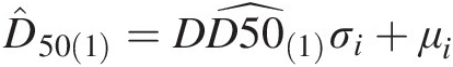 (12.12)
In Equation (12.12), {σi, μi}σiμi represents the seasonal deviation and seasonal mean for the forecasted month.


Applying the preceding five steps, Figure 12.13 plots the one-step ahead forecast with 5% and 95% VaRs of station D50 using the known information from D130. Table 12.13 lists the one-step ahead forecast results using meta-Gaussian and meta-Student t copulas. The results in Table 12.13 and Figure 12.13 indicate that the forecast follows the observed value well. The DO at the downstream location (D50) may be reasonably forecasted using the DO information at the upstream location (D130). In addition, results show that there is minimal difference in regard to the performance between the meta-Gaussian copula and the meta-Student t copula.

Figure 12.13 One-step ahead DO forecast, 5% and 95% VaRs for station D50 using DO information from D130.
Table 12.13. One-step ahead DO forecast for station D50 (mg/L).
| Month | Obs. | Gaussian copula | Student t copula | ||||
|---|---|---|---|---|---|---|---|
| Forecast | 5% VaR | 95% VaR | Forecast | 5% VaR | 95% VaR | ||
| Jan 2012 | 12.6 | 11.728 | 11.211 | 12.292 | 11.692 | 11.243 | 12.387 |
| Feb 2012 | 12 | 12.016 | 11.484 | 12.579 | 11.996 | 11.525 | 12.647 |
| Mar 2012 | 12.2 | 11.758 | 11.220 | 12.330 | 11.736 | 11.262 | 12.402 |
| Apr 2012 | 12.42 | 11.309 | 10.764 | 11.915 | 11.256 | 10.791 | 12.035 |
| May 2012 | 11.52 | 10.816 | 10.244 | 11.477 | 10.734 | 10.259 | 11.638 |
| Jun 2012 | 11.9 | 10.068 | 9.425 | 10.800 | 9.988 | 9.448 | 10.966 |
| Jul 2012 | 10.1 | 9.268 | 8.662 | 9.942 | 9.209 | 8.692 | 10.076 |
| Aug 2012 | 9 | 9.063 | 8.554 | 9.614 | 9.031 | 8.588 | 9.701 |
| Sep 2012 | 10.1 | 9.752 | 9.365 | 10.158 | 9.740 | 9.397 | 10.201 |
| Oct 2012 | 11.3 | 10.849 | 10.250 | 11.487 | 10.823 | 10.295 | 11.570 |
| Nov 2012 | 11.5 | 11.359 | 10.785 | 11.975 | 11.328 | 10.826 | 12.065 |
| Dec 2012 | 11.8 | 12.027 | 11.319 | 12.768 | 12.011 | 11.379 | 12.834 |
| Jan 2013 | 12.9 | 11.754 | 11.224 | 12.318 | 11.732 | 11.264 | 12.391 |
| Feb 2013 | 11.7 | 11.968 | 11.429 | 12.532 | 11.954 | 11.474 | 12.583 |
| Mar 2013 | 12.2 | 11.551 | 11.010 | 12.122 | 11.532 | 11.053 | 12.187 |
| Apr 2013 | 11.6 | 11.466 | 10.887 | 12.074 | 11.448 | 10.934 | 12.138 |
| May 2013 | 11.2 | 10.988 | 10.344 | 11.656 | 10.977 | 10.399 | 11.703 |
| Jun 2013 | 10.2 | 10.294 | 9.585 | 11.032 | 10.280 | 9.646 | 11.090 |
| Jul 2013 | 8.9 | 9.178 | 8.520 | 9.856 | 9.171 | 8.576 | 9.889 |
| Aug 2013 | 8.7 | 9.009 | 8.469 | 9.562 | 9.006 | 8.513 | 9.574 |
| Sep 2013 | 9.2 | 9.486 | 9.097 | 9.893 | 9.477 | 9.130 | 9.930 |
Using D130, C70, and D50 as Known Information to Forecast A90
Previously, we have illustrated the spatial–temporal dependence for the bivariate case (i.e., spatial dependence of D130 at the upstream and D50 at the downstream locations). Here, we will illustrate the multivariate spatial–temporal dependence. As shown in Figure 12.1, station A90 is the most downstream sampling location with stations D130, C70, and D50 as the upstream sampling locations. Here, we will show whether it is possible to perform a one-step ahead DO forecast for station A90 with the use of DOs at all three upstream sampling locations. Similar to the previous case, we will need to proceed as follows:
1. Compute the model error from the fitted univariate time series models for D130, C70, and D50.
2. Compute the probability for the model error obtained from Step 1.
3. Derive and compute P(A90| D130, C70, D50)PA90D130C70D50 from the fitted meta-Gaussian and meta-Student t copulas (the fitted copula parameters are listed in Table 12.12). As discussed previously, the conditional density function should follow the univariate Gaussian distribution (the meta-Gaussian copula) and univariate noncentral Student t distribution (meta-Student t copula), respectively.
In what follows, we will show the results of derived conditional distribution functions.
From the Meta-Gaussian Copula
 (12.13a)
 (12.13b)
In Equations (12.13), X1 = [Φ−1(UC70), Φ−1(UD50), Φ−1(D130)]TX1=Φ−1UC70Φ−1UD50Φ−1D130T is the conditioning vector; Σ11=10.580.720.5810.670.720.671;Σ12=Σ21T,Σ21=0.710.690.73;Σ22=1 .
.
As discussed in Chapter 7, and after some algebra, we have the following:
 (12.14a)
 (12.14b)
From the Meta-Student t Copula
Similar to the meta-Gaussian copula, the maginal CDF vector in Equation (12.13a) will be first transformed to Student t distribution with the degree of freedom νν. From Section 7.2.2 and Kotz and Nadarajah (2004), Equations (12.13) and (12.14) can be rewritten as follows:
 (12.15a)
 (12.15b)
 (12.15c)
In Equation (12.15), we have the following:
 (12.15e)
To this end, the conditional density function can be given as follows:
 (12.16)
As shown previously, X1=T−1Uc70νT−1UD50νT−1UD130νT;X2=T−1UA90∗ν .
.
From Equations (12.15) and (12.16), it is seen that the conditional variance is scalar. Equation (12.16) may also be called the scaled and shifted univariate Student t distribution.
Let tA90′=X2−μ2∣1Σ2∣112 ; tA90′
 will now follow the standard univariate Student t distribution: TtA90’ν2∣1
 .
.
Applying the previously discussed approach, Table 12.14 lists the one-step ahead forecast results. Figure 12.14 compares the one-step ahead forecast with the observed monthly DO values. The results again indicate that the DO forecasts for station A90 closely follow the corresponding observed DO values. The monthly DO at station A90 may be reasonably forecasted using the monthly DO at upstream locations (i.e., C70, D50, and D130). In addition, similar to the forecast at station D50, there is minimal difference in regard to the performance between the meta-Gaussian copula and the meta-Student t copula. We may safely choose the meta-Gaussian copula as the only candidate in this case.
Table 12.14. One-step ahead DO forecast for station A90 (mg/L).
| Month | Obs. | Gaussian copula | Student t copula | ||||
|---|---|---|---|---|---|---|---|
| Forecast | 5% VaR | 95% VaR | Forecast | 5% VaR | 95% VaR | ||
| Jan 2012 | 12.8 | 12.203 | 11.853 | 12.805 | 12.193 | 11.881 | 12.666 |
| Feb 2012 | 12.8 | 12.449 | 12.110 | 12.845 | 12.446 | 12.124 | 12.880 |
| Mar 2012 | 13.2 | 12.059 | 11.722 | 12.458 | 12.054 | 11.738 | 12.496 |
| Apr 2012 | 12.73 | 11.737 | 11.306 | 12.227 | 11.727 | 11.329 | 12.320 |
| May 2012 | 12.02 | 11.464 | 11.056 | 11.924 | 11.447 | 11.009 | 12.078 |
| Jun 2012 | 11.5 | 10.756 | 10.198 | 11.256 | 10.737 | 10.252 | 11.357 |
| Jul 2012 | 10 | 9.596 | 8.901 | 10.336 | 9.575 | 8.979 | 10.443 |
| Aug 2012 | 9.6 | 9.288 | 8.857 | 9.803 | 9.276 | 8.883 | 9.860 |
| Sep 2012 | 10.16 | 9.395 | 8.898 | 9.986 | 9.385 | 8.978 | 9.974 |
| Oct 2012 | 11.2 | 10.821 | 10.404 | 11.319 | 10.811 | 10.453 | 11.337 |
| Nov 2012 | 11.7 | 11.705 | 11.261 | 12.228 | 11.689 | 11.262 | 12.298 |
| Dec 2012 | 12.1 | 12.392 | 11.868 | 12.938 | 12.389 | 11.852 | 13.003 |
| Jan 2013 | 12.7 | 12.073 | 11.732 | 12.481 | 12.060 | 11.758 | 12.509 |
| Feb 2013 | 11.3 | 12.471 | 12.114 | 12.853 | 12.468 | 12.111 | 12.890 |
| Mar 2013 | 11.7 | 11.582 | 11.234 | 11.979 | 11.573 | 11.249 | 12.007 |
| Apr 2013 | 11.8 | 11.219 | 10.773 | 11.706 | 11.208 | 10.773 | 11.753 |
| May 2013 | 11.3 | 11.254 | 10.817 | 11.703 | 11.247 | 10.825 | 11.727 |
| Jun 2013 | 10.3 | 10.721 | 10.218 | 11.231 | 10.713 | 10.207 | 11.278 |
| Jul 2013 | 9 | 9.522 | 8.768 | 10.244 | 9.527 | 8.720 | 10.321 |
| Aug 2013 | 8.9 | 9.255 | 8.744 | 9.744 | 9.261 | 8.732 | 9.762 |
| Sep 2013 | 9.3 | 9.357 | 8.770 | 9.921 | 9.369 | 8.613 | 10.117 |

Figure 12.14 Comparison of one-step ahead forecast with the monthly observed DO values at station A90.
12.3 Dependence Study for the Chattahoochee River Watershed
According to the availability of the water quality dataset published by USGS, temperature, DO, and pH are selected for the upstream location, i.e., USGS2332017 (Belton Bridge). Besides temperature, DO, and pH, phosphorus is also selected for the downstream location, i.e., USGS2338000 (Whitesburg). For both locations, the period with continuous measurements are selected, that is, September 6–September 12. Similar to the case study for the Snohomish River watershed, we will first study the temporal dependence using the copula-based Markov process followed by the study of spatial dependence. Table 12.15 lists the water quality data selected, in which the water quality measurements of 2012 are used for forecast and calibration purposes.
Table 12.15. Monthly water quality measurements for the Chattahoochee River watershed.
| Time | USGS2332017 | USGS2338000 | |||||
|---|---|---|---|---|---|---|---|
| Temperature (°C) | DO (mg/L) | pH | Temperature (°C) | DO (mg/L) | pH | Phosphorus (mg/L) | |
| Sep-06 | 18.1 | 8.4 | 7.1 | 26.5 | 5.8 | 6.6 | 0.127 |
| Oct-06 | 9 | 10.9 | 7.2 | 23.4 | 8.3 | 7.5 | 0.056 |
| Nov-06 | 8 | 11.1 | 7.1 | 18.4 | 8.2 | 7 | 0.082 |
| Dec-06 | 7.2 | 11.2 | 7 | 13.1 | 9.2 | 7.2 | 0.05 |
| Jan-07 | 7.1 | 11.9 | 7.2 | 12.6 | 8.6 | 6.8 | 0.163 |
| Feb-07 | 3 | 13.3 | 7.3 | 11.5 | 10.8 | 7.1 | 0.065 |
| Mar-07 | 9.1 | 11.1 | 7 | 21.9 | 8.4 | 7.3 | 0.041 |
| Apr-07 | 11.4 | 11 | 7.2 | 17.4 | 7.8 | 7 | 0.081 |
| May-07 | 19.5 | 8.5 | 6.9 | 23 | 9.1 | 7.7 | 0.065 |
| Jun-07 | 21.3 | 7.1 | 7.4 | 25.9 | 6.3 | 6.9 | 0.104 |
| Jul-07 | 22.3 | 7.5 | 7.5 | 27.2 | 7 | 7.2 | 0.083 |
| Aug-07 | 26.1 | 6.5 | 7.4 | 29.3 | 6.3 | 7.1 | 0.055 |
| Sep-07 | 19.3 | 7.9 | 7.3 | 20.6 | 7.8 | 7 | 0.079 |
| Oct-07 | 17.6 | 8.4 | 6.9 | 20.9 | 7.9 | 6.8 | 0.07 |
| Nov-07 | 8 | 10.7 | 7.7 | 15.4 | 8.7 | 6.9 | 0.064 |
| Dec-07 | 12.7 | 10 | 7.2 | 16.7 | 9 | 7.2 | 0.038 |
| Jan-08 | 5 | 13.5 | 7.2 | 7.5 | 10.6 | 6.9 | 0.072 |
| Feb-08 | 8.2 | 10.9 | 7.1 | 12.8 | 9.2 | 6.7 | 0.069 |
| Mar-08 | 10.8 | 10.4 | 6.9 | 15.1 | 8.5 | 6.8 | 0.124 |
| Apr-08 | 12 | 9.8 | 7.2 | 15.3 | 8.5 | 6.6 | 0.059 |
| May-08 | 19.3 | 10.3 | 7.2 | 22.6 | 6.7 | 7 | 0.073 |
| Jun-08 | 26.9 | 7.4 | 7.2 | 26 | 6.9 | 7.2 | 0.067 |
| Jul-08 | 26.8 | 7.9 | 7.4 | 26.5 | 6.4 | 6.7 | 0.112 |
| Aug-08 | 23.8 | 7.3 | 7.1 | 27.6 | 6.5 | 6.7 | 0.061 |
| Sep-08 | 23.6 | 7.2 | 7.2 | 20.3 | 7.9 | 7.5 | 0.079 |
| Oct-08 | 11.6 | 10.8 | 7.2 | 20.4 | 7.6 | 7.3 | 0.08 |
| Nov-08 | 9.4 | 11.9 | 7.1 | 9.8 | 11.1 | 7.7 | 0.086 |
| Dec-08 | 6.5 | 12.8 | 7.1 | 12.5 | 8.8 | 6.8 | 0.256 |
| Jan-09 | 12.4 | 9.5 | 6.8 | 10.8 | 10.4 | 6.9 | 0.215 |
| Feb-09 | 4 | 12.3 | 7.3 | 10.3 | 10.1 | 7 | 0.149 |
| Mar-09 | 6.1 | 12.3 | 7.2 | 7.8 | 12.3 | 7.1 | 0.103 |
| Apr-09 | 11 | 10.6 | 7.2 | 15.5 | 7.8 | 7 | 0.074 |
| May-09 | 19.5 | 8 | 7 | 22.4 | 7.1 | 7.2 | 0.092 |
| Jun-09 | 21.9 | 8.4 | 7.1 | 25.6 | 6.5 | 7.2 | 0.095 |
| Jul-09 | 23.4 | 7.2 | 7.1 | 24.6 | 7.2 | 7.2 | 0.074 |
| Aug-09 | 26.3 | 7.9 | 7.2 | 27.4 | 7.2 | 7.3 | 0.096 |
| Sep-09 | 23.4 | 8.2 | 7.3 | 21.6 | 6.2 | 6.4 | 0.542 |
| Oct-09 | 15.8 | 8.7 | 7.2 | 15.1 | 8.4 | 7 | 0.103 |
| Nov-09 | 10.8 | 10.3 | 7.1 | 13.8 | 8.8 | 6.6 | 0.03 |
| Dec-09 | 9.4 | 9.8 | 7.2 | 11.6 | 9.2 | 6.9 | 0.035 |
| Jan-10 | 3.1 | 11.6 | 6.9 | 8 | 10.9 | 7 | 0.078 |
| Feb-10 | 5.3 | 10.9 | 7.3 | 6.6 | 11.8 | 6.8 | 0.051 |
| Mar-10 | 10.5 | 10 | 7.1 | 9.6 | 10.8 | 7 | 0.054 |
| Apr-10 | 16.9 | 9.6 | 7 | 14.6 | 9 | 7.1 | 0.078 |
| May-10 | 20.3 | 8.6 | 7 | 16.1 | 9.3 | 7 | 0.068 |
| Jun-10 | 23.9 | 7.2 | 6.9 | 25 | 7.3 | 7.2 | 0.092 |
| Jul-10 | 26.4 | 6.6 | 6.9 | 28.3 | 7.4 | 7.3 | 0.065 |
| Aug-10 | 24 | 7.3 | 7.1 | 25.4 | 7.6 | 7.1 | 0.056 |
| Sep-10 | 22.3 | 7.7 | 7 | 24.4 | 7.6 | 7.2 | 0.025 |
| Oct-10 | 15.2 | 9.8 | 7.2 | 18.3 | 9.2 | 7.4 | 0.054 |
| Nov-10 | 12.2 | 9.8 | 7.2 | 10.7 | 10.3 | 7.2 | 0.036 |
| Dec-10 | 10.8 | 9.1 | 6.9 | 5.6 | 12.2 | 7.2 | 0.032 |
| Jan-11 | 5.9 | 12.2 | 7.2 | 7 | 11.5 | 7.5 | 0.034 |
| Feb-11 | 7.1 | 11.6 | 7.2 | 7.3 | 11.2 | 7.3 | 0.062 |
| Mar-11 | 11.1 | 10.6 | 7 | 11.6 | 9.6 | 7 | 0.23 |
| Apr-11 | 13.7 | 10.7 | 7.1 | 14.6 | 8.8 | 7 | 0.08 |
| May-11 | 20.8 | 8.1 | 7.1 | 22.2 | 7.9 | 6.8 | 0.027 |
| Jun-11 | 23.2 | 7.8 | 7 | 25.9 | 6.8 | 6.6 | 0.115 |
| Jul-11 | 28.8 | 8.4 | 7.5 | 27.4 | 6.3 | 6.5 | 0.047 |
| Aug-11 | 23.6 | 7.1 | 7.3 | 27.3 | 6.6 | 6.6 | 0.063 |
| Sep-11 | 19.6 | 8.7 | 7.3 | 21.7 | 7.4 | 6.6 | 0.133 |
| Oct-11 | 16.6 | 9.6 | 7.2 | 17.7 | 8.6 | 6.8 | 0.029 |
| Nov-11 | 10.7 | 10.6 | 6.9 | 16.6 | 7 | 6.8 | 0.131 |
| Dec-11 | 9.5 | 10.5 | 6.9 | 10.8 | 10.3 | 6.7 | 0.034 |
| Jan-12 | 10 | 9.5 | 6.4 | 9.1 | 10.3 | 7.3 | 0.048 |
| Feb-12 | 10.2 | 10.9 | 7.2 | 11.2 | 10.1 | 6.6 | 0.042 |
| Mar-12 | 16.1 | 10.1 | 7 | 20.4 | 7.6 | 6.6 | 0.044 |
| Apr-12 | 18.8 | 8.8 | 7.1 | 18.3 | 8.4 | 6.9 | 0.057 |
| May-12 | 21.8 | 8.7 | 7.4 | 26.4 | 6.8 | 6.9 | 0.047 |
| Jun-12 | 26.4 | 8.4 | 7.1 | 25.8 | 6.9 | 7 | 0.122 |
| Jul-12 | 27.9 | 7.5 | 7.2 | 27.5 | 6.6 | 6.8 | 0.081 |
| Aug-12 | 23.7 | 8.2 | 7.3 | 25.3 | 7.1 | 6.8 | 0.066 |
| Sep-12 | 20 | 8.2 | 7 | 21.6 | 7.9 | 6.8 | 0.07 |
12.3.1 Temporal Dependence of the Univariate Water Quality Series with the Copula-Based Markov Process
Before we proceed with the study of temporal dependence with copula-based Markov process, we first investigate whether there exists seasonality in water quality parameters. Applying frequency analysis, Figures 12.15 and 12.16 plot the cumulative periodogram for the water quality parameters listed in Table 12.15. The plots show that a 12-month seasonality exists for water temperature and DO, while no obvious seasonality is observed for pH and phosphorus. Table 12.16 lists monthly average and standard deviations for DO and temperature with 12-month seasonality.

Figure 12.15 Cumulative periodograms of the upstream (Belton Bridge) water quality parameters.

Figure 12.16 Cumulative periodograms of the downstream (Whitesburg) water quality parameters.
Table 12.16. Monthly average and standard deviation for DO and temperature.
| Upstream | Downstream | |||||||
|---|---|---|---|---|---|---|---|---|
| DO (mg/L) | Temperature (oC) | DO (mg/L) | Temperature (oC) | |||||
| μμ | σσ | μμ | σσ | μμ | σσ | μμ | σσ | |
| Jan | 11.37 | 1.58 | 7.25 | 3.41 | 10.38 | 0.97 | 9.17 | 2.16 |
| Feb | 11.65 | 0.98 | 6.30 | 2.71 | 10.53 | 0.92 | 9.95 | 2.47 |
| Mar | 10.75 | 0.85 | 10.62 | 3.26 | 9.53 | 1.75 | 14.40 | 5.78 |
| Apr | 10.08 | 0.83 | 13.97 | 3.20 | 8.38 | 0.50 | 15.95 | 1.54 |
| May | 8.70 | 0.83 | 20.20 | 0.97 | 7.82 | 1.15 | 22.12 | 3.34 |
| Jun | 7.72 | 0.58 | 23.93 | 2.30 | 6.78 | 0.35 | 25.70 | 0.37 |
| Jul | 7.52 | 0.61 | 25.93 | 2.56 | 6.82 | 0.45 | 26.92 | 1.27 |
| Aug | 7.38 | 0.60 | 24.58 | 1.26 | 6.88 | 0.50 | 27.05 | 1.51 |
| Sep | 8.04 | 0.49 | 20.90 | 2.18 | 7.23 | 0.87 | 22.39 | 2.24 |
| Oct | 9.70 | 1.04 | 14.30 | 3.31 | 8.33 | 0.56 | 19.30 | 2.89 |
| Nov | 10.73 | 0.72 | 9.85 | 1.68 | 9.02 | 1.47 | 14.12 | 3.36 |
| Dec | 10.57 | 1.30 | 9.35 | 2.28 | 9.78 | 1.29 | 11.72 | 3.62 |
To study the temporal dependence, we will choose temperature, pH, and phosphorus at the downstream location (Whitesburg, USGS2338000) as an example. For the downstream temperature dataset, we will first perform the full deseasonalization. Applying the Markov order identification approach discussed in Section 9.5.2, Table 12.17 lists the Markov order identified for the selected downstream water quality time series using the meta-Gaussian copula for identification purposes.
Table 12.17. Markov order identification for the water quality time series.
| Variable | Ft, Ft − 1Ft,Ft−1 | Ft ∣ t − 1, Ft − 2 ∣ t − 1Ft∣t−1,Ft−2∣t−1 | Ft ∣ t − 1, t − 2, Ft − 3 ∣ t − 1, t − 2Ft∣t−1,t−2,Ft−3∣t−1,t−2 | Order | |||
|---|---|---|---|---|---|---|---|
| Τ | p-Val | τ | p-Val | τ | p-Val | ||
| Temperature | 0.22 | <0.01 | 0.24 | <0.01 | 0.078 | 0.34 | 2 |
| pH | 0.25 | <0.01 | 0.19 | 0.03 | 0.035 | 0.67 | 2 |
| Phosphorus | — | — | — | 0 | |||
The results in Table 12.17 indicate the following:
1. The deseasonalized temperature and pH may be modeled with a second-order copula-based Markov process.
2. Phosphorus may be considered a random variable; this result is in agreement with the cumulative periodogram plot for phosphorus shown in Figure 12.16.
Now we will only look into the serial dependence for the downstream temperature and pH. For the second-order process, the D-vine copula will again be applied with the Gumbel–Hougaard, Gaussian, Student t, Frank and Clayton copulas as candidates. Tables 12.18 and 12.19 list the results for the five copula candidates.
Table 12.18. Results from five copula candidates for the deseasonalized temperature series.
| T1 | Gumbel–Hougaard | Gaussian | Student t | Frank | Clayton |
|---|---|---|---|---|---|
| Parameters | 1.27 | 0.23 | [0.31, 6.24] | 1.67 | 0.43 |
| ML | 2.10 | 1.84 | 2.27 | 1.76 | 2.00 |
| AIC | –2.20 | –1.68 | –0.55 | –1.53 | –2.01 |
| T2 | Gumbel–Hougaard | Gaussian | Student t | Frank | Clayton |
|---|---|---|---|---|---|
| Parameters | 1.42 | 0.37 | [0.43, 10.36] | 2.60 | 2.28 |
| ML | 6.08 | 4.69 | 4.99 | 4.64 | 2.28 |
| AIC | –10.16 | –7.38 | –5.97 | –7.28 | –2.57 |
Table 12.19. Results from five copula candidates for the pH series.
| T1 | Gumbel–Hougaard | Gaussian | Student t | Frank | Clayton |
|---|---|---|---|---|---|
| Parameters | 1.33 | 0.33 | [0.46, 5.01] | 3.09 | 0.80 |
| ML | 3.04 | 3.63 | 4.72 | 4.41 | 5.06 |
| AIC | –4.08 | –5.26 | –5.45 | –6.82 | –8.12 |
| T2 | Gumbel–Hougaard | Gaussian | Student t | Frank | Clayton |
|---|---|---|---|---|---|
| Parameters | 1.18 | 0.31 | [0.34, 1E+7] | 2.25 | 2.37 |
| ML | 1.75 | 3.29 | 3.32 | 3.38 | 2.37 |
| AIC | –1.51 | –4.57 | –2.64 | –4.76 | –2.74 |
From the results in the tables, we see the following:
Deseasonal temperature (downstream): The Gumbel–Hougaard copula is selected as the best-fitted copula function for both T1 (lag-1 dependence) and T2 (conditional dependence of T|T-1 and T-2|T-1);
pH (downstream): The Clayton copula is selected as the best-fitted copula function for T1 (lag-1 dependence), while the Frank copula is selected for T2 (conditional dependence of T|T1 and T-2|T-1).
Using the fitted Gumbel–Gumbel copula model for the second-order deseasonalized temperature series and the Clayton–Frank model for the second-order pH series at the Whitesburg station, Figure 12.17 plots the range of simulated temperature and pH series. Figure 12.18 plots the lag-1 and lag-2 scatter plots to compare the serial dependence of observed versus simulated water quality series. Figure 12.17 shows that the observed water quality series falls into the range of simulation for both the monthly temperature and pH series. Figure 12.18 further indicates the lag-1 and lag-2 serial dependence are well captured by the fitted copula-based second-order Markov process.

Figure 12.17 Comparison of simulation versus observed measurements at the Whitesburg station.

Figure 12.18 Comparison of serial dependence of observed versus simulated monthly water quality time series (i.e., temperature [T] and pH) at the Whitesburg station.
We have shown that the copula-based second-order Markov process may be applied to model monthly temperature and pH at the Whitesburg station. Now we will evaluate the forecast/prediction capability of the copula-based Markov process through a one-step ahead forecast following the same procedure as discussed in the previous case study for the Snohomish River watershed. Figure 12.19 compares the one-step ahead forecast to the observed monthly temperature and pH for the first nine months of 2012. Figure 12.19 shows that the copula-based second-order Markov process provides reasonable forecasts for temperature and pH at the downstream Whitesburg station. The forecast results, listed in Table 12.20, show that maximum biases are 30% and 6% for temperature and pH, respectively.

Figure 12.19 Comparison of one-step forecast with the observed monthly water quality series.
Table 12.20. One-step ahead forecast results for temperature and pH at the Whitesburg station.
| Month | Temperature (°C) | pH | ||||||
|---|---|---|---|---|---|---|---|---|
| Obs. | Forecast | 5%VaR | 95% VaR | Obs. | Forecast | 5%VaR | 95%VaR | |
| Jan 2012 | 9.1 | 9.7 | 6.2 | 12.2 | 7.3 | 6.8 | 6.5 | 7.4 |
| Feb 2012 | 11.2 | 9.3 | 5.8 | 12.4 | 6.6 | 7.0 | 6.6 | 7.4 |
| Mar 2012 | 20.4 | 14.2 | 5.5 | 21.2 | 6.6 | 6.9 | 6.5 | 7.5 |
| Apr 2012 | 18.3 | 16.5 | 14.0 | 18.2 | 6.9 | 6.7 | 6.4 | 7.2 |
| May 2012 | 26.4 | 24.8 | 18.7 | 28.2 | 6.9 | 6.8 | 6.5 | 7.3 |
| Jun 2012 | 25.8 | 26.1 | 25.4 | 26.4 | 7 | 7.0 | 6.6 | 7.4 |
| Jul 2012 | 27.5 | 27.9 | 25.7 | 29.1 | 6.8 | 7.0 | 6.6 | 7.4 |
| Aug 2012 | 25.3 | 27.3 | 24.9 | 29.0 | 6.8 | 7.0 | 6.6 | 7.5 |
| Sep 2012 | 21.6 | 22.5 | 18.9 | 25.2 | 6.8 | 6.9 | 6.5 | 7.4 |
12.3.2 Spatial–Temporal Dependence of the Water Quality Time Series for the Chattahoochee River Watershed
As introduced in Section 12.1, the subwatershed upstream of the Belton Bridge station may be considered a forest watershed. With the major metropolitan area (the city of Atlanta) located between the Belton Bridge station and the Whitesburg station, the LULC is changed from mainly forest to urban developed watershed. To study the spatial dependence, we will use a major water quality parameter DO as an example.
As discussed in Section 12.3.1, there exists 12-month periodicity in the DO time series (Table 12.16, Figures 12.15 and 12.16). We will proceed with the same procedure as follows: (i) perform full deseasonalization on the upstream and downstream monthly DO series; (ii) build a univariate time series model for the deseasonalized DO series; (iii) study the spatial dependence through the fitted model residuals; and (iv) perform the one-step ahead DO forecast for Whitesburg with the use of DO at the upstream Belton Bridge station. Again, the monthly DO series before the year of 2012 is applied to build the time series model, and the monthly DO series after 2012 is used for forecast and validation purposes.
After full deseasonalization, Table 12.21 lists parameters estimated for the selected AR(2) model. Using the fitted-model residual, Table 12.21 lists the rank-based Kendall’s tau dependence measure of model residuals. The computed Kendall’s tau suggests that the fitted-model residual may be considered independent (with P-value = 0.82). Computing the Kendall’s tau for deseasonlized DO series, we have τ = − 0.08, P = 0.31τ=−0.08,P=0.31, which also indicates independence. The scatter plots shown in Figure 12.20 also indicate the independence pattern.
Table 12.21. Parameters estimated of the AR(2) model for the DO series.
| Station | Constant | ϕ1ϕ1 | ϕ2ϕ2 | σe2 | White noise check |
|---|---|---|---|---|---|
| Belton Bridge | 0.021 | 0.062 | 0.123 | 0.808 | H = 0, N(0, 0.8992)N00.8992 |
| Whitesburg | –0.0002 | 0.049 | 0.51 | 0.681 | H = 0, N(0, 0.8252)N00.8252 |
| τ = − 0.0198;τ=−0.0198; | P = 0.82 | ||||

Figure 12.20 Scatter plots for fitted-model residual and deaseasonalized DO series.
These results suggest that the change of LULC among the subwatersheds may significantly impact the spatial distribution pattern of water quality parameters that one may also expect. To this end, we will simply apply the product copula (i.e., independent copula: π = uvπ=uv) and the meta-Gaussian copula for the one-step ahead forecast. In addition, we compare the results from the copula to that computed from the univariate one-step ahead forecast for DO at Whitesburg. Figure 12.21 plots the one-step ahead forecast, and Table 12.22 lists the numerical forecast results. The one-step ahead forecast results show that the Gaussian copula yields similar forecast results as those from the univariate time series. The maximum absolute bias is about 24% (forecast of March 2012 from the Gaussian copula); while the product copula yields the largest root mean square error (RMSE) (0.84 mg/L). Overall, both the Gaussian copula and the product copula provide reasonable forecasts.

Figure 12.21 Comparison of observed DO with one-step ahead forecast through univariate, product, and Gaussian copulas.
Table 12.22. Comparison of forecast results.
| Month | Observed | 1-Step ahead DO forecast at Whitesburg (mg/L) | ||
|---|---|---|---|---|
| Univariate | Gaussian copula | Product copula | ||
| Jan 2012 | 10.3 | 9.72 | 9.75 | 8.38 |
| Feb 2012 | 10.1 | 10.72 | 10.73 | 9.78 |
| Mar 2012 | 7.6 | 9.42 | 9.44 | 7.77 |
| Apr 2012 | 8.4 | 8.24 | 8.25 | 7.45 |
| May 2012 | 6.8 | 7.17 | 7.16 | 6.64 |
| Jun 2012 | 6.9 | 6.77 | 6.76 | 6.75 |
| Jul 2012 | 6.6 | 6.62 | 6.62 | 6.34 |
| Aug 2012 | 7.1 | 6.96 | 6.94 | 6.91 |
| Sep 2012 | 7.9 | 7.03 | 7.03 | 6.65 |
| Maximum bias | 23.9% | 24.2% | 18.6% | |
| RMSE (mg/L) | 0.742 | 0.749 | 0.844 | |
Above all, we have shown that even for the subwatershed with significantly different LULC, the copula method may still be applied to investigate the spatial–temporal dependence and provide reasonable forecasting results that may be useful for the watershed engineers to make proper judgment ahead.
In water quality studies, there exists one more type of dependence that is similar to that in at-site flood, rainfall, or drought frequency analysis. In water quality studies, the at-site dependence study may provide important information. Given the water quality information at Whitesburg, it will be useful if we can responsibly forecast phosphorus with the commonly monitored temperature, DO, and pH. Thus, in the following section, we will focus on the at-site multivariate water quality study.
12.4 At-Site Multivariate Water Quality Dependence Study
For the at-site multivariate water quality dependence study, we will choose the Whitesburg station as a case study. From the previous sections, we have shown temperature and pH may be modeled using the copula-based second-order Markov process, while phosphorus may be considered a random variable (Table 12.17). DO at Whitesburg may be modeled with the AR(2) univariate time series, so we will first evaluate whether temperature and pH may also be modeled with the AR(2) univariate time series. The results listed in Table 12.23 indicate that pH may be modeled using the AR(2) model, while the deseasonalized temperature may be modeled with ARMA(2,1) instead. Table 12.24 lists the Kendall’s tau correlation matrix for the residuals computed from the time series model of temperature (T), pH, DO, and observed phosphorus (P), which may be considered a random variable. Table 12.24 indicates the negative correlation of P with both DO and pH, while P is nearly independent of T.
Table 12.23. Classic time series modeling results for temperature and pH.
| Model | White noise check | |
|---|---|---|
| Temperature | ARMA(2,1) | |
C=−0.04,ϕ1=0.86,ϕ2=0.07,θ1=−1,σe2=0.50 | H0 = 0, P = 0.56H0=0,P=0.56 | |
| pH | AR(2) | |
C=3.61,ϕ1=0.18,ϕ2=0.31,σe2=0.07 | H0 = 0, P = 0.85H0=0,P=0.85 |
Table 12.24. Rank-based Kendall’s tau correlation matrix.
| DO | pH | T | P | |
|---|---|---|---|---|
| DO | 1 | 0.33 | –0.39 | –0.19 |
| pH | 0.33 | 1 | –0.14 | –0.16 |
| T | –0.39 | –0.14 | 1 | 0.04 |
| P | –0.19 | –0.16 | 0.04 | 1 |
With the preceding information, we will build two models, i.e., (i) a full model of f(DO, pH, T, P)fDOpHTP; and (ii) a reduced model of f(DO, pH, P)fDOpHP.
Full model. For the full model, we will simply apply the meta-Gaussian and meta-Student t copula to illustrate the analysis. Table 12.25 lists the parameters estimated for the full model.
Table 12.25. Parameter estimated for the full model using meta-elliptical copulas.
| Meta-Gaussian | Meta-Student t | |||||||
|---|---|---|---|---|---|---|---|---|
| DO | pH | T | P | DO | pH | T | P | |
| DO | 1 | 0.49 | –0.56 | –0.33 | 1 | 0.57 | –0.63 | –0.40 |
| pH | 0.49 | 1 | –0.18 | –0.33 | 0.57 | 1 | –0.27 | –0.41 |
| T | –0.56 | –0.18 | 1 | 0.06 | –0.63 | –0.27 | 1 | 0.14 |
| P | –0.33 | –0.33 | 0.06 | 1 | –0.40 | –0.41 | 0.14 | 1 |
| ν = 1.12 × 10⁷ν=1.12×10⁷ | ||||||||
Using DO, PH, and T as conditioning variables, Figure 12.22 compares the phosphorus forecast with its observations. The comparison shows that the phosphorus observations are within the range of 5% and 95% VaRs. The obvious differences are seen between the forecasts and observations for the very high and very low sampled phosphorus values.

Figure 12.22 Comparison of the one-step ahead forecast with the phosphorus samplings.
Reduced model. In the case of reduced model, Table 12.26 tabulates the rank-based Kendall correlation matrix. As seen in Table 12.26, the negative relation is found between phosphorus and DO as well as phosphorus and pH. Meta-elliptical and vine copulas will be applied to evaluate the reduced model.
Table 12.26. Rank-based Kendall’s tau correlation matrix for reduced model.
| DO | pH | Phosphorus | |
|---|---|---|---|
| DO | 1.00 | 0.33 | –0.19 |
| pH | 0.33 | 1.00 | –0.16 |
| Phosphorus | –0.19 | –0.16 | 1.00 |
Applying the meta-elliptic copulas, Table 12.27 tabulates the estimated parameters for meta-Gaussian and meta-Student t copulas with the one-step ahead forecast plotted in Figure 12.23. Comparing Figure 12.23 to Figure 12.22, we may reach the following conclusions:
i. For the meta-Gaussian model, the median forecast and 5% (95% VaRs) yield similar results for both full and reduced models.
ii. For the meta-Student t model, the median forecast and 5% VaRs yield similar results for both the full and reduce models. However, there exist noticeable differences in regard to the 95% VaRs estimated from the full and reduced models.
iii. The observations fall into the region bounded by 5% and 95% VaRs.
Table 12.27. Parameters estimated from meta-Gaussian and meta-Student t copulas.
| Meta-Gaussian | Meta-Student t | |||||
|---|---|---|---|---|---|---|
| DO | pH | Phosphorus | DO | pH | Phosphorus | |
| DO | 1.00 | 0.49 | –0.33 | 1.00 | 0.55 | –0.38 |
| Ph | 0.49 | 1.00 | –0.33 | 0.55 | 1.00 | –0.38 |
| Phosphrous | –0.33 | –0.33 | 1.00 | –0.38 | –0.38 | 1.00 |
| ν = 10.56ν=10.56 | ||||||

Figure 12.23 Comparison of the one-step ahead forecast with the phosphorus samplings for the reduced model using meta-elliptical copulas.
Applying the vine copulas, we choose either DO or pH as the center. Results indicate that phosphorus may be studied only using DO or pH rather than both of the variables as follows:
pH as center: The Clayton copula is selected to study DO and pH, while the Gaussian copula is selected to study DO and phosphorus for the first level T1. The rank-based correlation for the second-level T2 is computed as –0.03 with a P-value of 0.75 for pH|DO and P|DO.
DO as center: With the Clayton copula selected to study DO and pH, the Gaussian copula is again found as the proper copula to study pH and phosphorus for the first-level T1. The rank-based correlation of T2 is computed as –0.08 with a P-value of 0.35 for DO|pH and P|pH.
Thus, the model may be further reduced to the bivariate model with the use of the meta-Gaussian copula for (P, DO with parameter ρ = − 0.326ρ=−0.326) or (P, pH with parameter ρ = − 0.332ρ=−0.332). Figure 12.24 plots the one-step ahead forecast of phosphorus using pH and DO, respectively.

Figure 12.24 Comparison of the one-step ahead forecast with the phosphorus sampling for reduced model through (a) pH and (b) DO.
Figure 12.24 again shows the similar results comparing the full model and reduced model with the use of meta-elliptical copulas. To further compare all three models, Table 12.28 lists the results of comparison, which indicate that (i) the largest error occurs for June forecast from both full and reduced models; (ii) the full model results in the smallest RMSE compared to the reduced models; (iii) comparing the further reduced bivariate model using either pH or DO with the reduced model using pH, DO, and temperature through meta-elliptic copulas, there exist minimal differences; and (iv) the negative relations between pH and phosphorous, as well as DO and phosphorous, are in line with natural phenomena.
Table 12.28. Prediction results from full and reduced model.
| Observations | Full model | Reduced model | ||||
|---|---|---|---|---|---|---|
| Meta-Gaussian | Meta-Student t | Meta-Gaussian | Meta-Student t | Through pH | Though DO | |
| Jan, 0.048 | 0.055 | 0.052 | 0.059 | 0.058 | 0.059 | 0.067 |
| Feb, 0.042 | 0.081 | 0.083 | 0.088 | 0.090 | 0.087 | 0.080 |
| Mar, 0.044 | 0.082 | 0.085 | 0.093 | 0.097 | 0.090 | 0.084 |
| Apr, 0.057 | 0.054 | 0.052 | 0.066 | 0.066 | 0.067 | 0.068 |
| May, 0.047 | 0.063 | 0.062 | 0.072 | 0.072 | 0.069 | 0.074 |
| Jun, 0.122 | 0.059 | 0.057 | 0.066 | 0.066 | 0.068 | 0.066 |
| Jul, 0.081 | 0.068 | 0.067 | 0.076 | 0.076 | 0.077 | 0.071 |
| Aug, 0.066 | 0.072 | 0.072 | 0.073 | 0.073 | 0.077 | 0.068 |
| Sep, 0.07 | 0.059 | 0.057 | 0.066 | 0.065 | 0.074 | 0.060 |
| RMSE | 0.005 | 0.003 | 0.027 | 0.028 | 0.031 | 0.020 |
| Max absolute error | 0.063 | 0.065 | 0.056 | 0.056 | 0.054 | 0.056 |
| Min absolute error | 0.003 | 0.004 | 0.004 | 0.005 | 0.004 | 0.002 |
12.5 Summary
In this chapter, we have introduced the copula application in water quality analysis. Two types of watersheds have been considered: (1) natural watershed and (2) urban watershed. The two case studies indicate the following:
I. The copula-based Markov process (CMP) is more robust compared to the classic time series with Gaussian innovations. The serial dependence structure may be well preserved through D-vine copula. The simulation study shows the ability to apply CMP for water quality management. The forecast study indicates the good forecast ability of CMP. In addition, compared to the urban watershed (the watershed in Georgia), the forecast accuracy of CMP is higher for the natural watershed (the watershed in Washington ).
II. In the case of the spatial analysis for the natural watershed in Washington, the spatial distribution pattern of DO is well preserved. Given the characteristic of the water quality data information (i.e., monthly data), the meta-elliptic copulas perform very well to capture the spatial dependence as well as the one-step ahead water quality forecast.
III. In the case of at-site multivariate water quality frequency analysis for the watershed in Georgia, the forecast ability is acceptable but not as good as that for the natural watershed in Washington. The largest forecast error (phosphorus) occurs in June for both full and reduced models. This may be due to the following: (1) the human activities are usually more active during the late spring/early summer (i.e., agricultural practice); (2) runoff into the system from rainfall events or irrigation may bring more nutrients into the system, which result in high values; and (3) with more information of human activity, the forecast ability of the model may be improved.
IV. For the watershed in Georgia, there is no obvious dependence structure between the upstream (Belton Bridge) and downstream (Whitesburg) subwatersheds due to the significant change of LULC (i.e., natural [or forest] for the upstream subwatershed, while urban for the downstream [the city of Atlanta]). In addition, the behavior of phosphorus at the downstream (i.e., random) may be considered another indicator of disturbance due to the human activities within the watershed.
V. Overall, the copula-based approach provides a rule-of-thumb for watershed engineers in regard to water quality parameters that need to be monitored and to make the protocol for management purposes.
VI. Due to the limitations of the water quality data, the monthly water quality data have been applied for both of the case-study watersheds, and the monthly model can be easily converted to the model for water quality with higher sampling frequencies (i.e., weekly, daily, etc.) to provide more immediate evaluation for decision making (e.g., algal control protocol through water quality measurement).