Abstract
In this chapter, we focus on the copula applications to at-site bivariate/trivariate drought analysis. In a case study, drought variables are separated from long-term daily streamflow series, i.e., drought severity, drought duration, drought interarrival time, and maximum drought intensity. Drought severity and duration are applied for bivariate drought frequency analysis. Drought severity, duration, and maximum intensity are applied for trivariate drought frequency analysis. The Archimedean, meta-elliptical, and vine copulas are adopted for the bivariate/trivariate analyses. The case study shows that the copula approach may be properly applied for drought analysis.
13.1 Introduction
Droughts may be identified with the following five types: (1) agricultural drought, (2) meteorological drought, (3) hydrological drought, (4) groundwater drought, and (5) social-economic drought. The commonly applied drought indices include Palmer drought severity index (PDSI; Palmer, 1965), crop moisture index (CMI; Palmer, 1968), standard precipitation index (SPI; McKee et al., 1993), and standard runoff index (SRI; Shukla and Wood, 2008). There are many other indices discussed and compared in an extensive review paper by Mishra and Singh (2010). According to the drought index applied, drought events may then be determined using the run theory proposed by Yevjevich (1967). For each drought event, there are three characteristics: drought severity (S: total deficit), drought duration (D), and drought intensity (the average intensity is usually considered: I = S/D). There is one more variable for two consecutive independent drought events: interarrival time (IT). The IT represents the time span from the onset of the first drought event to the onset of the second drought event (i.e., dry period + wet period). Figure 13.1 depicts the drought characteristics.

Figure 13.1 Schematic of drought characteristics.
13.2 Copula Applications in Drought Studies
Conventionally, drought has been studied with the use of univariate frequency analysis (Van Rooy, 1965; Palmer, 1968; Santos, 1983; Rao and Padmanabhan, 1984; Voss et al. 2002; among others). With the increasing popularity of copula application in hydrology and water resources engineering, copulas have been applied to model bivariate and trivariate drought frequency analyses (Chen et al., 2013; Yoo et al., 2013; Hao and AghaKouchak, 2014; Janga et al., 2014; AghaKouchak, 2015; Salvadori and De Michele, 2015; Zhang et al., 2015; Kwak et al., 2016; Hao et al., 2016; Tu et al., 2016; among others). Here we first review some recent studies, followed by examples applying copulas to drought analysis.
Kao and Govindaraju (2010) proposed a joint deficit index (JDI) for drought analysis. In their study, monthly precipitation and streamflow data, computed from daily values, were applied for meteorological and hydrological drought analysis with the temporal window ranging from one month to 12 months. As a result, a 12-dimensional empirical copula was constructed to compute the Kendall distribution of KC(t) = P(C(u1, u2, …u12) ≤ t)KCt=PCu1u2…,u12≤t. The JDI was defined using the standardized normal distribution transformation as follows: JDI = Φ−1[KC(t)]JDI=Φ−1KCt. In their method, there was no need to separate the drought events, based on a separation criterion (e.g., the threshold for flow computed from the flow-duration curve). Using the trivariate Plackett copula with the genetic algorithm for parameter estimation, Song and Singh (2010a) investigated the dependence among three drought characteristics (i.e., severity, duration, and interarrival time) using the trivariate Plackett copula. In their study, the Weibull distribution was applied to model drought duration and interarrival time, while the gamma distribution was applied to model drought severity. Song and Singh (2010b) investigated the drought frequency with the meta-elliptical copula.
Madadgar and Moradkhani (2013) investigated drought under climate change by readjusting the SDI (streamflow drought index) with different moving windows. In their study, the impact of climate change on drought was studied through the future climate scenarios generated from the General Circulation Models (GCMs). The Student t and Gumbel–Hougaard copulas were applied to study the dependence structure.
Chen et al. (2013) studied four drought characteristics, using the SPI index. The Archimedean and meta-elliptical copulas were chosen as the candidates to model the association of drought characteristics, i.e., drought severity, drought duration, interval time, and minimum SPI.
Rather than using the well-known drought characteristics of drought duration, drought severity, and interarrival time, Xu et al. (2015) applied the affected area, drought duration, and drought severity as the drought indicators for bivariate and trivariate drought frequency analyses to capture the spatial–temporal variability. Similar to other studies, drought variables were considered as random variables.
13.3 Hydrological Drought with the Use of Daily Streamflow: A Case Study
In this case study, we illustrate the copula application using daily streamflow (from December 1, 1942, to February 7, 2017) from the Nueces River near Tilden. Located in Texas, the Nueces River is about 315 miles in length and 16,800 square miles in drainage area (average annual runoff of about 620,000 acre-feet). The Nueces River flows through the central and southern parts of Texas and empties into the Gulf of Mexico. The unregulated USGS gauging station near Tilden (28°18’31”N, 98°33’25”W, i.e., USGS08194500) is located upstream (i.e., west) of the first major reservoir (i.e., the Chock Canyon Reservoir). In addition, as stated in the Handbook of Texas, the Nueces River watershed is predominantly a rural area, with the only metropolis of Corpus Christi located at the mouth (Texas State Historical Association, n.d.).
Daily (or monthly) streamflow statistics were also readily available from the USGS website that can be applied to determine the threshold of drought severity. Among all the available daily steamflow data from December 1, 1942, to February 2, 2017, daily streamflow data from August 19, 2009, to September 30, 2009, were not available.
13.3.1 Determination of Drought Severity, Duration, and Interarrival Time
The theory of runs, proposed by Yevjevich (1967), was used to determine the drought severity (i.e., total flow deficit in the case of hydrological drought). Following Yevjevich (1967), the threshold equation can be written as follows:
 (13.1)
where μi, σiμi,σi represent the estimated long-term mean and standard deviation (daily or monthly), depending on the streamflow records.
Given the high fluctuation of daily streamflow, we will use the long-term daily average streamflow as a threshold. Additionally, following Zelenhasic and Salvai (1987), (a) minor drought events were ignored under the condition of Si ≤ 0.005 max (S), i = 1, 2, ..NSi≤0.005maxS,i=1,2,…,N, where N represents the total number of drought events identified and S represents the drought severity; and (b) the two consecutive drought events were pooled into a single drought event if the interevent wet period was relatively short and the ratio of surplus of pervious drought severity was small, the pooled event can be given as follows:
where Si, Si + 1Si,Si+1 represent drought severity of two consecutive drought events; Di, Di + 1Di,Di+1 represent the drought duration of two consecutive drought events; and SPi, i + 1SPi,i+1 represents the total amount of streamflow above the threshold in the wet period between the two consecutive droughts.
The rules to pool the events are as follows:
i. The consecutive drought events are pooled into one drought event, if the interevent wet period is less than seven days.
ii. To pool the consecutive drought events if the ratio Δ ≤ 0.05Δ≤0.05 in Equation (13.2) such that the total surplus in the interevent period cannot relieve the dry condition.
To further illustrate the process, we show a simple example using daily streamflow from June 20, 1943, to May 2, 1944. Table 13.1 lists observed daily streamflow and its difference from the long-term daily average. The surplus of daily streamflow is in bold Italic. Figure 13.2 graphs the streamflow time series and the differences from daily thresholds. It is seen from Figure 13.2 that there existed flow deficit for most of the time in the period from June 20, 1943, to May 2, 1944.
Table 13.1. Sample daily streamflow and the difference from the long-term daily average.
| Time | (1) | (2) | Time | (1) | (2) | Time | (1) | (2) |
|---|---|---|---|---|---|---|---|---|
| 6/20/1943 | 260 | –475.14 | 10/4/1943 | 527 | –17.39 | 1/18/1944 | 0.3 | –77.15 |
| 6/21/1943 | 134 | –569.28 | 10/5/1943 | 231 | –238.80 | 1/19/1944 | 0.2 | –67.45 |
| 6/22/1943 | 249 | –415.00 | 10/6/1943 | 192 | –267.71 | 1/20/1944 | 0.1 | –71.63 |
| 6/23/1943 | 214 | –331.42 | 10/7/1943 | 368 | –189.20 | 1/21/1944 | 0.1 | –73.92 |
| 6/24/1943 | 118 | –346.54 | 10/8/1943 | 476 | –492.46 | 1/22/1944 | 0.1 | –58.30 |
| 6/25/1943 | 91 | –298.27 | 10/9/1943 | 512 | –699.65 | 1/23/1944 | 0.1 | –58.64 |
| 6/26/1943 | 58 | –299.96 | 10/10/1943 | 440 | –575.82 | 1/24/1944 | 0.1 | –71.94 |
| 6/27/1943 | 35 | –329.05 | 10/11/1943 | 272 | –1,264.61 | 1/25/1944 | 0.1 | –74.61 |
| 6/28/1943 | 21 | –368.70 | 10/12/1943 | 169 | –969.71 | 1/26/1944 | 0.1 | –78.00 |
| 6/29/1943 | 13 | –519.24 | 10/13/1943 | 118 | –924.32 | 1/27/1944 | 0.1 | –87.55 |
| 6/30/1943 | 8.6 | –606.69 | 10/14/1943 | 84 | –917.10 | 1/28/1944 | 0.1 | –95.74 |
| 7/1/1943 | 5.7 | –651.45 | 10/15/1943 | 72 | –1,014.33 | 1/29/1944 | 0.1 | –98.22 |
| 7/2/1943 | 4 | –731.88 | 10/16/1943 | 58 | –1,224.35 | 1/30/1944 | 0.1 | –80.38 |
| 7/3/1943 | 2.7 | –860.08 | 10/17/1943 | 36 | –1,291.34 | 1/31/1944 | 0.1 | –66.76 |
| 7/4/1943 | 1.8 | –880.55 | 10/18/1943 | 22 | –1,212.70 | 2/1/1944 | 0.2 | –60.67 |
| 7/5/1943 | 1.1 | –1,032.43 | 10/19/1943 | 15 | –1,352.55 | 2/2/1944 | 0.1 | –57.44 |
| 7/6/1943 | 0.7 | –1,106.26 | 10/20/1943 | 10 | –1,029.42 | 2/3/1944 | 0.1 | –51.09 |
| 7/7/1943 | 0.5 | –1,059.12 | 10/21/1943 | 6.8 | –881.09 | 2/4/1944 | 0.1 | –61.35 |
| 7/8/1943 | 0.4 | –1,035.25 | 10/22/1943 | 5 | –769.01 | 2/5/1944 | 0.1 | –76.43 |
| 7/9/1943 | 0.4 | –993.28 | 10/23/1943 | 4 | –699.60 | 2/6/1944 | 0.1 | –86.45 |
| 7/10/1943 | 0.7 | –877.82 | 10/24/1943 | 2.7 | –668.94 | 2/7/1944 | 0.1 | –78.81 |
| 7/11/1943 | 0.6 | –737.09 | 10/25/1943 | 1.6 | –744.00 | 2/8/1944 | 0.1 | –71.32 |
| 7/12/1943 | 0.3 | –662.59 | 10/26/1943 | 1 | –703.39 | 2/9/1944 | 0.1 | –62.20 |
| 7/13/1943 | 314 | –284.57 | 10/27/1943 | 0.7 | –650.11 | 2/10/1944 | 0.1 | –51.69 |
| 7/14/1943 | 676 | 200.28 | 10/28/1943 | 0.5 | –633.03 | 2/11/1944 | 0 | –48.69 |
| 7/15/1943 | 304 | –165.87 | 10/29/1943 | 0.3 | –597.11 | 2/12/1944 | 0 | –52.46 |
| 7/16/1943 | 424 | –176.39 | 10/30/1943 | 0.2 | –559.78 | 2/13/1944 | 0 | –52.09 |
| 7/17/1943 | 608 | 121.57 | 10/31/1943 | 0.1 | –540.33 | 2/14/1944 | 0 | –51.05 |
| 7/18/1943 | 495 | –43.63 | 11/1/1943 | 0.1 | –612.66 | 2/15/1944 | 0 | –49.88 |
| 7/19/1943 | 285 | –258.77 | 11/2/1943 | 0.1 | –587.60 | 2/16/1944 | 0 | –46.82 |
| 7/20/1943 | 285 | –158.28 | 11/3/1943 | 0.1 | –536.40 | 2/17/1944 | 0 | –43.75 |
| 7/21/1943 | 315 | –32.26 | 11/4/1943 | 0.1 | –479.11 | 2/18/1944 | 0 | –41.93 |
| 7/22/1943 | 268 | –32.48 | 11/5/1943 | 119 | –301.67 | 2/19/1944 | 0 | –40.49 |
| 7/23/1943 | 149 | –134.54 | 11/6/1943 | 150 | –221.10 | 2/20/1944 | 0 | –41.64 |
| 7/24/1943 | 72 | –174.14 | 11/7/1943 | 53 | –272.51 | 2/21/1944 | 0 | –57.31 |
| 7/25/1943 | 36 | –176.77 | 11/8/1943 | 22 | –268.47 | 2/22/1944 | 0 | –90.26 |
| 7/26/1943 | 20 | –198.86 | 11/9/1943 | 10 | –256.47 | 2/23/1944 | 0 | –320.83 |
| 7/27/1943 | 13 | –231.18 | 11/10/1943 | 5.7 | –257.31 | 2/24/1944 | 0 | –628.09 |
| 7/28/1943 | 8.8 | –229.18 | 11/11/1943 | 3.5 | –261.08 | 2/25/1944 | 0 | –421.89 |
| 7/29/1943 | 6.8 | –231.50 | 11/12/1943 | 75 | –184.71 | 2/26/1944 | 0 | –292.50 |
| 7/30/1943 | 5.2 | –239.47 | 11/13/1943 | 121 | –99.92 | 2/27/1944 | 0 | –195.38 |
| 7/31/1943 | 3.8 | –255.87 | 11/14/1943 | 87 | –99.26 | 2/28/1944 | 0 | –126.72 |
| 8/1/1943 | 2.6 | –246.38 | 11/15/1943 | 61 | –76.85 | 2/29/1944 | 0 | –72.65 |
| 8/2/1943 | 1.7 | –219.91 | 11/16/1943 | 49 | –61.05 | 3/1/1944 | 0 | –101.54 |
| 8/3/1943 | 1.1 | –207.64 | 11/17/1943 | 34 | –69.37 | 3/2/1944 | 0 | –92.08 |
| 8/4/1943 | 0.8 | –198.74 | 11/18/1943 | 133 | –8.79 | 3/3/1944 | 0 | –80.73 |
| 8/5/1943 | 0.6 | –211.95 | 11/19/1943 | 268 | 96.80 | 3/4/1944 | 0 | –79.80 |
| 8/6/1943 | 0.5 | –219.54 | 11/20/1943 | 102 | –95.73 | 3/5/1944 | 0 | –80.14 |
| 8/7/1943 | 0.4 | –214.45 | 11/21/1943 | 36 | –220.37 | 3/6/1944 | 0 | –97.36 |
| 8/8/1943 | 0.4 | –208.52 | 11/22/1943 | 17 | –208.21 | 3/7/1944 | 0 | –235.27 |
| 8/9/1943 | 0.4 | –236.16 | 11/23/1943 | 10 | –181.14 | 3/8/1944 | 0 | –237.32 |
| 8/10/1943 | 0.3 | –320.24 | 11/24/1943 | 7.2 | –172.71 | 3/9/1944 | 0 | –192.98 |
| 8/11/1943 | 0.2 | –315.58 | 11/25/1943 | 5 | –179.02 | 3/10/1944 | 0.1 | –154.09 |
| 8/12/1943 | 0.2 | –294.99 | 11/26/1943 | 3.6 | –174.14 | 3/11/1944 | 0 | –116.15 |
| 8/13/1943 | 0.2 | –355.40 | 11/27/1943 | 3.5 | –159.81 | 3/12/1944 | 0 | –100.34 |
| 8/14/1943 | 0.1 | –366.51 | 11/28/1943 | 4.6 | –130.02 | 3/13/1944 | 0 | –101.19 |
| 8/15/1943 | 0.1 | –441.86 | 11/29/1943 | 4 | –116.98 | 3/14/1944 | 0 | –99.40 |
| 8/16/1943 | 0.1 | –377.74 | 11/30/1943 | 4.6 | –123.94 | 3/15/1944 | 0 | –92.68 |
| 8/17/1943 | 0.1 | –279.99 | 12/1/1943 | 4.8 | –128.70 | 3/16/1944 | 0 | –93.21 |
| 8/18/1943 | 0.1 | –236.28 | 12/2/1943 | 3.1 | –139.21 | 3/17/1944 | 0 | –91.94 |
| 8/19/1943 | 0 | –228.42 | 12/3/1943 | 3.1 | –129.13 | 3/18/1944 | 0 | –89.59 |
| 8/20/1943 | 0 | –343.15 | 12/4/1943 | 12 | –115.58 | 3/19/1944 | 0.1 | –90.63 |
| 8/21/1943 | 0 | –457.47 | 12/5/1943 | 80 | –40.66 | 3/20/1944 | 40 | –51.56 |
| 8/22/1943 | 0 | –445.06 | 12/6/1943 | 180 | 72.08 | 3/21/1944 | 216 | 111.83 |
| 8/23/1943 | 0 | –395.05 | 12/7/1943 | 260 | 162.21 | 3/22/1944 | 144 | 52.34 |
| 8/24/1943 | 0 | –354.06 | 12/8/1943 | 146 | 59.89 | 3/23/1944 | 62 | –14.97 |
| 8/25/1943 | 0 | –321.86 | 12/9/1943 | 90 | 12.07 | 3/24/1944 | 27 | –43.74 |
| 8/26/1943 | 0 | –299.22 | 12/10/1943 | 45 | –28.66 | 3/25/1944 | 9.4 | –58.92 |
| 8/27/1943 | 0 | –279.80 | 12/11/1943 | 30 | –43.74 | 3/26/1944 | 4.8 | –65.01 |
| 8/28/1943 | 0 | –273.29 | 12/12/1943 | 31 | –40.46 | 3/27/1944 | 37 | –23.18 |
| 8/29/1943 | 0 | –263.71 | 12/13/1943 | 25 | –42.85 | 3/28/1944 | 140 | 85.44 |
| 8/30/1943 | 0 | –254.53 | 12/14/1943 | 16 | –56.60 | 3/29/1944 | 245 | 182.52 |
| 8/31/1943 | 0 | –237.63 | 12/15/1943 | 9.5 | –70.99 | 3/30/1944 | 196 | 120.86 |
| 9/1/1943 | 0 | –268.43 | 12/16/1943 | 7.7 | –70.07 | 3/31/1944 | 102 | 32.65 |
| 9/2/1943 | 0 | –289.05 | 12/17/1943 | 5.7 | –71.02 | 4/1/1944 | 60 | –9.06 |
| 9/3/1943 | 159 | –462.74 | 12/18/1943 | 4 | –73.18 | 4/2/1944 | 39 | –50.95 |
| 9/4/1943 | 505 | –218.31 | 12/19/1943 | 2.9 | –81.02 | 4/3/1944 | 29 | –62.65 |
| 9/5/1943 | 749 | 2.21 | 12/20/1943 | 2.1 | –91.09 | 4/4/1944 | 19 | –68.82 |
| 9/6/1943 | 1130 | 382.68 | 12/21/1943 | 1.8 | –94.72 | 4/5/1944 | 15 | –68.02 |
| 9/7/1943 | 1760 | 1056.62 | 12/22/1943 | 1.6 | –116.84 | 4/6/1944 | 11 | –74.92 |
| 9/8/1943 | 1690 | 953.12 | 12/23/1943 | 1.4 | –116.90 | 4/7/1944 | 6.8 | –82.04 |
| 9/9/1943 | 352 | –414.57 | 12/24/1943 | 1.1 | –101.90 | 4/8/1944 | 5 | –90.34 |
| 9/10/1943 | 186 | –626.36 | 12/25/1943 | 0.9 | –92.09 | 4/9/1944 | 3.5 | –97.91 |
| 9/11/1943 | 348 | –229.78 | 12/26/1943 | 0.9 | –89.79 | 4/10/1944 | 2 | –107.93 |
| 9/12/1943 | 305 | –238.43 | 12/27/1943 | 0.7 | –82.95 | 4/11/1944 | 1 | –132.69 |
| 9/13/1943 | 146 | –725.07 | 12/28/1943 | 0.6 | –74.80 | 4/12/1944 | 0.7 | –139.90 |
| 9/14/1943 | 60 | –952.46 | 12/29/1943 | 0.5 | –90.51 | 4/13/1944 | 0.4 | –116.94 |
| 9/15/1943 | 31 | –931.12 | 12/30/1943 | 0.4 | –91.35 | 4/14/1944 | 0.3 | –90.52 |
| 9/16/1943 | 25 | –997.26 | 12/31/1943 | 0.4 | –89.75 | 4/15/1944 | 0.2 | –86.47 |
| 9/17/1943 | 22 | –921.83 | 1/1/1944 | 0.5 | –93.26 | 4/16/1944 | 0.1 | –81.40 |
| 9/18/1943 | 14 | –766.21 | 1/2/1944 | 0.5 | –86.10 | 4/17/1944 | 0.1 | –89.15 |
| 9/19/1943 | 10 | –578.15 | 1/3/1944 | 0.4 | –85.01 | 4/18/1944 | 0.1 | –105.27 |
| 9/20/1943 | 7.7 | –440.76 | 1/4/1944 | 0.4 | –78.94 | 4/19/1944 | 0.1 | –105.92 |
| 9/21/1943 | 5.4 | –681.06 | 1/5/1944 | 0.4 | –94.52 | 4/20/1944 | 0.1 | –91.85 |
| 9/22/1943 | 3.8 | –1,140.30 | 1/6/1944 | 0.3 | –106.63 | 4/21/1944 | 0.1 | –126.40 |
| 9/23/1943 | 2.4 | –1,072.43 | 1/7/1944 | 0.3 | –116.32 | 4/22/1944 | 0.1 | –179.66 |
| 9/24/1943 | 87 | –1,349.54 | 1/8/1944 | 0.3 | –139.38 | 4/23/1944 | 0 | –218.81 |
| 9/25/1943 | 93 | –1,060.46 | 1/9/1944 | 0.4 | –183.61 | 4/24/1944 | 0 | –210.94 |
| 9/26/1943 | 62 | –714.50 | 1/10/1944 | 0.4 | –168.02 | 4/25/1944 | 0 | –244.29 |
| 9/27/1943 | 46 | –563.73 | 1/11/1944 | 0.4 | -131.69 | 4/26/1944 | 0 | –365.98 |
| 9/28/1943 | 24 | –530.45 | 1/12/1944 | 0.4 | -113.08 | 4/27/1944 | 0 | –432.56 |
| 9/29/1943 | 116 | –394.19 | 1/13/1944 | 0.5 | -112.36 | 4/28/1944 | 0 | –394.68 |
| 9/30/1943 | 75 | –507.08 | 1/14/1944 | 0.6 | -103.62 | 4/29/1944 | 0 | –414.73 |
| 10/1/1943 | 101 | –566.52 | 1/15/1944 | 0.5 | -95.25 | 4/30/1944 | 0 | –661.52 |
| 10/2/1943 | 451 | –202.83 | 1/16/1944 | 0.4 | -89.38 | 5/1/1944 | 0 | –733.76 |
| 10/3/1943 | 629 | 20.89 | 1/17/1944 | 0.3 | -88.86 | 5/2/1944 | 245 | –339.09 |
Note: (1): Observed daily streamflow in cfs; (2) difference from the long-term daily average using observed-daily average in cfs in which the negative values represent the flow deficit.

Figure 13.2 Daily streamflow and its difference from the long-term daily threshold from June 20, 1943, to May 2, 1944.
Without either ignoring or pooling drought events, Table 13.2 lists the drought events by adding the continuous flow deficit (negative flow differences). In addition, before pooling the drought events together, we compute the maximum drought deficit, which is 2.36E+05 cfs.day from all the available daily streamflow data investigated in the case study. With the maximum drought deficit, the deficit less than 0.005 max (deficit) = 0.005(2.36 × 10⁵) = 1181.2 cfs. day0.005maxdeficit=0.0052.36×105=1181.2cfs.day. With this criterion, the minor drought event from March 23, 1944, to March 27, 1944, is ignored, which is in bold Italic (Table 13.2). After ignoring minor droughts, Table 13.3 lists the remaining drought events. These remaining drought events are then further pooled using the rules of pooling discussed earlier. In addition, the last two droughts also need to be pooled, since Δ = 0.03 ≤ 0.05Δ=0.03≤0.05. Finally, all the individual droughts in Table 13.3 need to be pooled into one drought as follows:
Severity = 89257.53 cfs.day; Duration = 293 days; Inter-arrival time=334 days;
Starting time = 06/20/1943; Ending time = 05/02/1944.
Table 13.2. Drought identified before ignoring minor droughts and pooling droughts.
| Start | End | Severity (cfs.day) | Duration (day) | Interarrival (day) | Surplus (cfs.day) | Interevent time (days) |
|---|---|---|---|---|---|---|
| 06/20/1943 | 07/13/1943 | 15,471.67 | 24 | 28 | 200.28 | 4 |
| 07/18/1943 | 09/04/1943 | 12,740.57 | 49 | 53 | 2,394.63 | 4 |
| 09/09/1943 | 10/02/1943 | 16,605.10 | 24 | 25 | 20.89 | 1 |
| 10/04/1943 | 11/18/1943 | 25,782.17 | 46 | 47 | 96.80 | 1 |
| 11/20/1943 | 12/05/1943 | 2,315.34 | 16 | 20 | 306.24 | 1 |
| 12/10/1943 | 03/20/1944 | 10,267.52 | 102 | 113 | 164.16 | 11 |
| 03/23/1944 | 03/27/1944 | 205.82 | 5 | 9 | 421.46 | |
| 04/01/1944 | 05/02/1944 | 6,075.16 | 32 | 41 | 5,709.02 | 9 |
Table 13.3. Drought events by ignoring minor droughts.
| Start | End | Severity (cfs.day) | Duration (day) | Surplus (cfs.day) | Interevent (day) | Eq. (12.2) : ΔEq.12.2:Δ |
|---|---|---|---|---|---|---|
| 06/20/1943 | 07/13/1943 | 15,471.67 | 24 | 200.28 | 4 | 0.02 |
| 07/18/1943 | 09/04/1943 | 12,740.57 | 49 | 2,394.63 | 4 | 0.14 |
| 09/09/1943 | 10/02/1943 | 16,605.10 | 24 | 20.89 | 1 | 0.00 |
| 10/04/1943 | 11/18/1943 | 25,782.17 | 46 | 96.80 | 1 | 0.04 |
| 11/20/1943 | 12/05/1943 | 2,315.34 | 16 | 306.24 | 1 | 0.03 |
| 12/10/1943 | 03/20/1944 | 10,267.52 | 102 | 164.16 | 11 | 0.03 |
| 04/01/1944 | 05/02/1944 | 6,075.16 | 32 | 5,709.02 | 9 | 0.85 |
Using the identification procedure for drought events explained previously, we identified a total of 115 drought events. Table 13.4 lists the statistics of these identified drought events. As shown in Table 13.4, the fluctuations of drought variables are significant with a heavy tail. The drought events, such identified, are assumed as independent random variables. To further ensure the assumption, we will apply correlation by lag, as shown in Figure 13.3. The autocorrelation function plot with lag indicates that there is no serial dependence within each individual drought variable. As a result, drought variables can be considered as random variables for analysis. More specifically, drought variables are assumed to be continuous random variables throughout the analysis.
Table 13.4. Statistics of identified drought events.
| Mean | Std. | Skewness | Kurtosis | |
|---|---|---|---|---|
| Severity (S: cfs.day) | 63189.05 | 83782.42 | 2.42 | 9.73 |
| Duration (D: days) | 183.24 | 229.57 | 2.20 | 8.60 |
| Interarrival time (IT: days) | 263.90 | 286.64 | 2.29 | 9.16 |

Figure 13.3 Check for independence of drought variables.
13.3.2 Univariate Drought Frequency Analysis
Before we proceed to the bivariate and trivariate drought analyses, we will first perform univariate drought frequency analysis. The fitted parametric univariate distribution will be applied for risk analysis. To study the univariate drought frequency analysis, drought variables are conventionally assumed as continuous random variables. It is also known that there may be ties that commonly exist in drought duration and drought interarrival time variables. To avoid the impact of ties in the univariate analysis, the parametric univariate distribution is fitted to the unique values (e.g., if there is more than one 30-day duration drought, only one 30-day duration will be used for fitting the univariate distribution). We obtain that (i) if there is no tie in drought severity, all 115 drought severity values are applied for univariate analysis; (ii) there are 15 values that are repeated more than once for the drought duration, and 93 unique duration values are applied for univariate analysis; (iii) there are 13 values that are repeated more than once for drought interarrival times, and 98 unique interarrival time values are applied for the univariate analysis.
Based on the previous studies, the following parametric univariate distributions are considered as candidates: gamma, exponential, and Weibull distributions. In addition, the log-normal distribution has been commonly applied to model drought severity (i.e., streamflow deficit), while the Weibull distribution has been commonly applied to model drought duration and drought interarrival time. Table 13.5 lists the fitted univariate distributions as well as the formal goodness-of-fit (GoF) statistics using the Kolmogorov–Smirnov (KS) test. Figure 13.4 compares the parametric marginal distributions with the empirical distributions. From Table 13.5, it is seen that the log-normal (for severity and duration) and exponential (for interarrival time) distributions yield the smallest KS test statistics (i.e., the smallest distance between the parametric and empirical distributions). However, comparisons in Figure 13.4 show that (i) in the case of drought severity and drought duration, the Weibull distribution fits the upper tail better than the lognormal distribution; and (ii) in the case of drought interarrival time, there is minimal difference in fitting the upper tail for log-normal and Weibull distributions. To comply with the conventional univariate drought analysis, we will use the conventional marginal distributions for illustration, i.e., log-normal distribution for drought severity and Weibull distribution for drought duration and drought interarrival time. One other reason of applying the conventional distributions is that both log-normal and Weibull distributions pass the formal GoF KS test.
Table 13.5. Fitted univariate distribution and GoF test results.
| Severity (cfs.day) | Duration (days) | Interarrival time (days) | ||||
|---|---|---|---|---|---|---|
| Parameters | GoF [S, P]a | Parameters | GoF [S, P] | Parameters | GoF [S, P] | |
| Log-normal | [10.20, 1.46] | [0.042, 0.68] | [4.69, 1.32] | [0.04, 0.93] | [5.17, 1.03] | [0.059, 0.33] |
| Exponential | 63189 | [0.17, 0] | 216.18 | [0.12, 0.01] | 285.6 | [0.046, 0.66] |
| Weibull | [54413, 0.78] | [0.074, 0.067] | [203.8, 0.89] | [0.079, 0.077] | [291.6, 1.05] | [0.064, 0.24] |
Note: a S: KS test statistic, P: P-value computed using the parametric bootstrap method.

Figure 13.4 Fitted parametric marginal distributions versus empirical distribution.
13.3.3 Bivariate Drought Frequency Analysis
Fitting Copula Functions to Bivariate Drought Variables
Using the identified drought events, Figure 13.5 plots show the scatter plots of the paired random variables. Figure 13.5 clearly shows the positive dependence between drought severity and drought duration; between drought severity and drought interarrival time; as well as between drought duration and drought interarrival time.

Figure 13.5 Scatter plots of paired drought variables.
As introduced in Chapter 3, we will investigate the dependence separately from the marginals. The empirical marginals (i.e., using the Weibull plotting position formula) are applied to study the dependence among drought variables. The parametric marginal distributions, fitted in the previous section, will be applied for risk analysis through joint (and/or conditional) return periods. In addition, we will choose the Archimedean and meta-elliptical copulas for the bivariate drought analysis, while only meta-elliptical copulas will be chosen for trivariate drought analysis. Given the positive dependence structure between drought variables, the selected Archimedean copulas are the Gumbel–Hougaard (which belongs to the extreme value family), Clayton, and Frank copulas. One may also choose other Archimedean copulas as candidates. The Gaussian and Student t copulas are selected as candidates from the meta-elliptical family.
Applying the pseudo-MLE to the bivariate drought variables, Table 13.6 lists the estimated copula parameters as well as the GoF test results through the improved Rosenblatt transform following the procedures discussed in Section 3.8.3 (i.e., the SnB test; Genest, et al., 2007) with the following steps briefly outlined:
i. For d-dimensional random variables u = [u1, u2, …, ud]u=u1u2…ud; setting Z = [Z1, Z2, …, Zd],Z=Z1Z2…Zd, where Z1=u1=F1x1;Z2=∂Cu1u2∂u1;…,Zd=∂Cd−1u1…ud∂u1∂u2…∂ud−1∂Cd−1u1…ud−1∂u1∂u2…∂ud−1
 The null hypothesis is that u = [u1, u2, …, ud]~Cθ ⇒ Z = [Z1, Z2, …, Zd]u=u1u2…ud~Cθ⇒Z=Z1Z2…Zd are independent.
ii. Compute the test statistic using

 (13.3).
iii. Generate random variables from the fitted copula function with the same sample size as the sample data.
iv. Reestimate the copula parameters from the tested copula function and recompute the test statistics.
v. Repeat steps ii–iv for a large number of times (N) and approximate the P-value using
Pvalue=1N∑k=1N1Sn,kB∗>SnB,
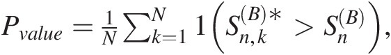 where Sn,kB∗
 represents the test statistic from step iv.


From Table 13.6 we obtain that (i) all the copula candidates from Archimedean and meta-elliptical families may be applied to model drought severity (S) and drought duration (D) as well as drought severity (S) and drought interarrival time (INT); (ii) the Gumbel–Hougaard and Guassian copulas are the only two copula functions that may be applied to model drought duration and drought interarrival time.
Table 13.6. Parameters estimated and GoF test for copula candidates.
| S and D | S and INT | D and INT | ||||
|---|---|---|---|---|---|---|
| (1) | (2) | (1) | (2) | (1) | (2) | |
| GHa | [6.2, 157.31] | [0.17, 0.24] | [3.30, 90.00] | [0.06, 0.81] | [3.97, 109.02] | [0.27, 0.08] |
| Clayton | [4.11, 92.71] | [0.26, 0.08] | [2.10, 49.23] | [0.21, 0.13] | [2.80, 64.50] | [0.42, 0.02] |
| Frank | [18.88, 126.33] | [0.17, 0.23] | [11.21, 80.73] | [0.10, 0.56] | [14.76, 80.73] | [0.32, 0.04] |
| Gaussian | [0.95, 137.11] | [0.33, 0.15] | [0.87, 80.77] | [0.08, 0.71] | [0.91, 99.78] | [0.26, 0.10] |
| Student t | (0.95, 1.47)b | [0.24, 0.10] | (0.88, 5.79) | [0.10, 0.54] | (0.92, 4.99) | [0.31, 0.04] |
| 144.68c | 83.59 | 104.73 | ||||
Notes: (1) estimated parameter and CL; (2) SnB test statistics and P-value;
a GH represents the Gumbel–Hougaard copula, bcorrelation and degree of freedom, c CL for Student t copula.
Joint and Conditional Return Period for Bivariate Drought Analysis
In this section, we will apply the Gumbel–Hougaard copula (which belongs to the extreme value family) and the Gaussian copula to investigate risk through joint and conditional return periods. Here, we will only focus on drought severity and drought duration.
Joint Return Period of Bivariate Drought Analysis
As discussed in Section 3.10.2, the bivariate joint return period may be represented with either the “AND” case or “OR” case. Here we will focus on the “AND” case only. Equation (3.139) in Chapter 3 can be revised as follows:
 (13.4)
where E(INT) represents the expected drought interarrival time in years, E(INT) = 0.723 year.
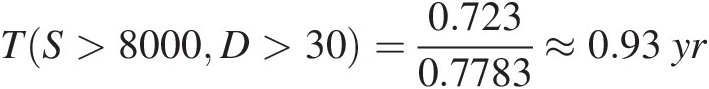
Using Equation (3.139), Table 13.7 lists the “AND” case joint return periods with the fitted parametric marginal distributions. To further illustrate the computation, we will show how to compute the return period for T(S>8000 cfs. day, D>30 days)TS>8000cfs.dayD>30days:
FS(S < 8000) = 0.2035FSS<8000=0.2035 from the fitted log-normal distribution S~LN2(10.1992, 1.4614)S~LN210.19921.4614.
FD(D < 30) = 0.1661FDD<30=0.1661 from the fitted Weibull distribution D~Weibull(203.80, 0.8903)D~Weibull203.800.8903.
FS, D(S ≤ 8000, D ≤ 30) = C(0.2035, 0.1661; θ = 6.2015) = 0.1479FS,DS≤8000D≤30=C0.20350.1661θ=6.2015=0.1479 from the fitted Gumbel–Hougaard copula for drought severity and drought duration.
The exceedance probability:
FS>8000D>30=1−FS8000−FD30+CFSFD=1−0.2035−0.1661+0.1479=0.7783
The “AND” case joint return period TS>8000D>30=0.7230.7783≈0.93yr
 .
.


Figure 13. 6 shows the Joint return period of the “AND” case for drought severity and drought duration.
Table 13.7. Joint return period of drought severity and duration (“AND” case).

Figure 13.6 Joint return period of the “AND” case for drought severity and drought duration.
Conditional Return Period of Bivariate Drought Variables
There are two commonly applied approaches to study the conditional return period:
T(X1>x1| X2>x2)TX1>x1X2>x2 and T(X1>x1| X2 = x2)TX1>x1X2=x2. Here, we will investigate both conditional return periods for drought severity and drought duration, with the use of drought duration as the conditioning variable.
T(S>s| D>d)TS>sD>d In this case, the exceedance conditional probability of S given D exceeding a given duration (d) can be written through the copula as follows:
 (13.5)
The conditional return period can then be written as follows:
 (13.6)
Equation (13.5) may also tell whether there exists the right tail increasing (RTI) property. The RTI property exists if the conditional exceedance probability is a nondecreasing function of drought duration for all drought severity values.
Using Equations (13.5) and (13.6) and the Gumbel–Hougaard copula as an illustrative example, Table 13.8 lists the conditional exceedance probability and conditional return period. Figure 13.7 plots the conditional exceedance probability and conditional return period. From Table 13.8 and Figure 13.7, it is seen that the exceedance probability is a nondecreasing function of duration, i.e., with the increase of drought duration, the exceedance probability of S>s|D>d is nondecreasing. The RTI property indicates that it is more likely for the drought severity exceeding a given threshold conditioned on a higher drought duration than that conditioned on a lower drought duration. Using S > 8000 cfs.day in Table 13.8 as an example, we have the following:

From Table 13.8 and Figure 13.7, it is also seen that for a given drought duration, the exceedance probability decreases with the increase of drought severity. To illustrate the computation, we will show the procedure to compute P(S>8000| D>30)PS>8000D>30 and T(S>8000| D>30)TS>8000D>30:
Previously we have computed P(S>8000, D>30) = 0.7783PS>8000D>30=0.7783 for the “AND” case.
The exceedance conditional probability is as follows: PS>8000D>30=PS>8000D>30PD>30=0.77831−0.1661=0.933

The conditional return period is as follows:
TS>8000D>30=EINT1−FD30PS>8000.D>30=0.7231−0.16610.7783≈1.11yr


Table 13.8. Conditional exceedance probability and conditional return period using drought duration as the conditioning variable.
| D (days) P(S>s| D>d)PS>sD>d | D (days) T(S>s| D>d)TS>sD>d | ||||||||||||
|---|---|---|---|---|---|---|---|---|---|---|---|---|---|
| 30 | 120 | 365 | 520 | 700 | 1,120 | 30 | 120 | 365 | 520 | 700 | 1,120 | ||
| 8,000 | 0.93 | 1.00 | 1.00 | 1.00 | 1.00 | 1.00 | 1.11 | 2.52 | 20.82 | 72.27 | 291.60 | 6586.07 | |
| 28,000 | 0.59 | 0.87 | 1.00 | 1.00 | 1.00 | 1.00 | 1.77 | 2.88 | 20.82 | 72.27 | 291.60 | 6586.07 | |
| S | 92,000 | 0.24 | 0.37 | 0.92 | 1.00 | 1.00 | 1.00 | 4.34 | 6.75 | 22.54 | 72.46 | 291.61 | 6586.07 |
| (cfs.day) | 180,000 | 0.12 | 0.18 | 0.52 | 0.87 | 1.00 | 1.00 | 8.98 | 13.97 | 40.30 | 82.84 | 292.81 | 6586.08 |
| 300,000 | 0.06 | 0.09 | 0.27 | 0.49 | 0.88 | 1.00 | 17.55 | 27.32 | 78.54 | 146.80 | 330.78 | 6586.36 | |
| 800,000 | 0.01 | 0.02 | 0.05 | 0.10 | 0.20 | 0.87 | 85.66 | 133.33 | 383.31 | 714.17 | 1434.63 | 7600.17 | |

Figure 13.7 Conditional exceedance probability and conditional return period of S>s ∣ D>dS>s∣D>d.
T(S>s| D = d)TS>sD=d. In this case, the drought duration is the fixed conditioning variable. The exceedance conditional probability may be written as follows:
 (13.7)
The conditional return period can then be written as follows:
 (13.8)
According to Nelson (2006), the stochastic increasing (SI) property exists if P(S>s| D = d)PS>sD=d is a nondecreasing function of drought duration for all drought severity values.
Using Equations (13.7) and (13.8) and the Gumbel–Hougaard copula as an illustrative example, Table 13.9 lists the exceedance conditional probability and conditional return period. Figure 13.8 plots the exceedance probability and conditional return period. Figure 13.8 clearly shows that for D = d, the exceedance probability P(S>s| D = d)PS>sD=d is a nondecreasing function of drought duration, i.e., P(S>s| D = d1) ≤ P(S>s| D = d2), d1 < d2PS>sD=d1≤PS>sD=d2,d1<d2.
Table 13.9. Exceedance conditional probability and conditional return period of S>s ∣ D = dS>s∣D=d.
| D (days) P(S>s| D = d)PS>sD=d | D (days) T(S>s| D = d)TS>sD=d | ||||||||||
|---|---|---|---|---|---|---|---|---|---|---|---|
| 30 | 120 | 365 | 520 | 700 | 30 | 120 | 365 | 520 | 700 | ||
| 8000 | 0.36 | 0.99 | 1.00 | 1.00 | 1.00 | 2.02 | 0.73 | 0.72 | 0.72 | 0.72 | |
| 28000 | 0.00 | 0.29 | 1.00 | 1.00 | 1.00 | 286.86 | 2.45 | 0.72 | 0.72 | 0.72 | |
| S | 92000 | 2.73E-06 | 0.00 | 0.57 | 0.98 | 1.00 | 2.65E+05 | 1.60E+03 | 1.27 | 0.74 | 0.72 |
| (cfs.day) | 180000 | 2.08E-08 | 3.45E-06 | 0.01 | 0.39 | 0.97 | 3.48E+07 | 2.10E+05 | 67.70 | 1.83 | 0.74 |
| 300000 | 2.78E-10 | 4.61E-08 | 1.44E-04 | 0.01 | 0.43 | 2.60E+09 | 1.57E+07 | 5.01E+03 | 80.12 | 1.67 | |
| 800000 | 1.33E-14 | 2.19E-12 | 6.85E-09 | 4.32E-07 | 3.82E-05 | 5.43E+13 | 3.31E+11 | 1.06E+08 | 1.67E+06 | 1.89E+04 | |

Dynamic Return Period for a Given Drought Episode
In the previous sections, we have investigated the joint and conditional return periods of bivariate drought variables, namely drought severity and drought duration. Following De Michele et al. (2013), we will investigate the evolution of drought within a given drought event (or simply called drought episode). It is worth mentioning that the copula function fitted to the drought severity and drought duration will not be applicable here. The empirical copula will be applied to study the dynamic return period for the given drought episode.
As discussed in De Michele et al. (2013), the dynamic return period is estimated through the Survival Kendall Distribution (also called DSKRP). As introduced in Section 4.5.1, the Kendall distribution may be considered as univariate realization of the copula function. In the case of bivariate analysis, the Kendall distribution may be simply written as follows:
and the survival Kendall distribution K¯Ct may be written as follows:
 (13.10)
In Equation (13.10), C¯ represents the survival copula, and FXi¯xi=1−FXixi,i=1,2
 .
.
The DSKRP can then be written as follows:
 (13.11)
In Equation (13.11), μμ represents the average interarrival time of the drought event (μ = 0.723 yr)μ=0.723yr).
Furthermore, to investigate the DSKRP for a given drought episode, the average running drought intensity (I) will be applied. The average running drought intensity is computed as the average drought deficit starting from the initiation of a drought episode until day k into the drought. With this in mind, the new bivariate drought variable is given by pair as (Ik, k), k = 1, 2, …, mIkk,k=1,2,…,m, where m represents the total number of days of the drought episode. To illustrate the DSKRP method, we will use the recent 21-day drought episode identified (i.e., September 7–27, 2016) as an example. Table 13.10 lists the daily streamflow and streamflow deficit during this dry period.
Table 13.10. Daily streamflow and flow deficit from September 7 to September 27, 2016.
| Date | Flow (cfs) | Deficit (cfs) | IkIk |
|---|---|---|---|
| 7-Sep-2016 | 444 | 259.38 | 259.38 |
| 8-Sep-2016 | 154 | 582.88 | 421.13 |
| 9-Sep-2016 | 102 | 664.57 | 502.28 |
| 10-Sep-2016 | 73 | 739.36 | 561.55 |
| 11-Sep-2016 | 56 | 521.78 | 553.60 |
| 12-Sep-2016 | 46 | 497.43 | 544.24 |
| 13-Sep-2016 | 36 | 835.07 | 585.78 |
| 14-Sep-2016 | 29 | 983.46 | 635.49 |
| 15-Sep-2016 | 24 | 938.12 | 669.12 |
| 16-Sep-2016 | 20 | 1,002.26 | 702.43 |
| 17-Sep-2016 | 17 | 926.83 | 722.83 |
| 18-Sep-2016 | 15 | 765.21 | 726.36 |
| 19-Sep-2016 | 13 | 575.15 | 714.73 |
| 20-Sep-2016 | 11 | 437.46 | 694.93 |
| 21-Sep-2016 | 8.8 | 677.66 | 693.78 |
| 22-Sep-2016 | 7.4 | 1,136.70 | 721.46 |
| 23-Sep-2016 | 6.5 | 1,068.33 | 741.86 |
| 24-Sep-2016 | 5.5 | 1,431.04 | 780.15 |
| 25-Sep-2016 | 6.4 | 1,147.06 | 799.46 |
| 26-Sep-2016 | 74 | 702.50 | 794.61 |
| 27-Sep-2016 | 366 | 243.73 | 768.38 |
As introduced earlier, the running average Ik can be computed as follows:

For example, for the drought period of day 3, we have the following: I3=259.38+582.88+664.573=502.28cfs .
.
Figure 13.9 plots the flow deficit running average, as well as DSKRP and return period computed from the univariate flow deficit (RPFD) for the recent dry period. The plot on the left shows that the running average fluctuates within the drought episode. This fluctuation may reflect the severity of the state of drought on a given day. The plot on the right shows the DSKRP and the RPFD. It shows that within the drought episode, DSKRP and RPFD for the state of drought share a similar pattern and reflect the fluctuation of flow deficit. Table 13.11 lists the computed survival Kendall distribution and the corresponding DSKRP. As an illustration, here we will show how to compute DSKRP for (I1, 1) = (259.38, 1)I11=259.381:
1. To compute the exceedance empirical marginal probability, use Weibull plotting position formula as follows:
FIk¯I1=1−FIkIk≤I1=1−121+1≈0.9545;F¯k1=1−121+1≈0.9545.
2. To compute the empirical survival copula, i.e., C¯
 , apply the following formula:
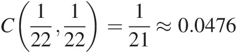
C¯FIkI1Fk1=FIk¯I1+F¯k1−1+CFIkI1Fk1=0.9545+0.9545−1+C122122=0.9545+0.9545−1+0.0476≈0.9567Here, C(FIk(I1), Fk(1))CFIkI1Fk1 is estimated using the empirical copula formula given as Equation (2.59). The first pair (I1, 1) = (259.38, 1)I11=259.381 is the smallest pair among all (Ik, k), k = 1, 2, …Ikk,k=1,2,…. and we have C122122=121≈0.0476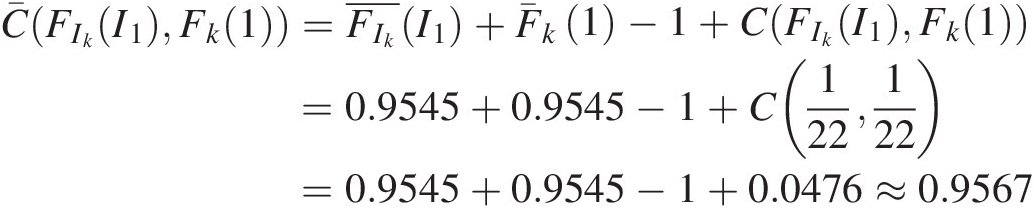
 .
.
3. To compute the empirical survival Kendall distribution K¯C
 , Equation (13.10) is applied to compute the empirical survival Kendall distribution. Again using C¯FIkI1Fk1
 as an example, we have C¯FIkI1Fk1≈0.957
 , which is the largest one among all the pairs, then, K¯C0.957=121+1≈0.045
 .
.
4. To compute DSKRP and RPFD, DSKRP = E(INT)/1−K¯Ct
 ; RPFD=E(INT)/[1-FIkFIk].


Figure 13.9 Flow deficit running average and DSKRP for 2016 event from September 7–27.
Table 13.11. Results for estimating DSKRP and RPFD.
| Date | IkIk | FIkFIk (cfs) | FkFk | Rank (Ik, k)Ikk | C(FIk, Fk)CFIkFk | ĈFIkFk | K¯Ct | DSKRP (yrs) | RPFD (yrs) |
|---|---|---|---|---|---|---|---|---|---|
| 7-Sep-16 | 259.38 | 0.045 | 0.045 | 1 | 0.048 | 0.957 | 0.045 | 0.757 | 0.757 |
| 8-Sep-16 | 421.13 | 0.091 | 0.091 | 2 | 0.095 | 0.913 | 0.091 | 0.795 | 0.795 |
| 9-Sep-16 | 502.28 | 0.136 | 0.136 | 3 | 0.143 | 0.870 | 0.136 | 0.837 | 0.837 |
| 10-Sep-16 | 561.55 | 0.273 | 0.182 | 4 | 0.190 | 0.736 | 0.273 | 0.994 | 0.994 |
| 11-Sep-16 | 553.60 | 0.227 | 0.227 | 4 | 0.190 | 0.736 | 0.273 | 0.994 | 0.936 |
| 12-Sep-16 | 544.24 | 0.182 | 0.273 | 4 | 0.190 | 0.736 | 0.273 | 0.994 | 0.884 |
| 13-Sep-16 | 585.78 | 0.318 | 0.318 | 7 | 0.333 | 0.697 | 0.318 | 1.060 | 1.060 |
| 14-Sep-16 | 635.49 | 0.364 | 0.364 | 8 | 0.381 | 0.654 | 0.364 | 1.136 | 1.136 |
| 15-Sep-16 | 669.12 | 0.409 | 0.409 | 9 | 0.429 | 0.610 | 0.409 | 1.224 | 1.224 |
| 16-Sep-16 | 702.43 | 0.545 | 0.455 | 10 | 0.476 | 0.476 | 0.455 | 1.326 | 1.591 |
| 17-Sep-16 | 722.83 | 0.682 | 0.500 | 11 | 0.524 | 0.342 | 0.500 | 1.446 | 2.272 |
| 18-Sep-16 | 726.36 | 0.727 | 0.545 | 12 | 0.571 | 0.299 | 0.727 | 2.651 | 2.651 |
| 19-Sep-16 | 714.73 | 0.591 | 0.591 | 11 | 0.524 | 0.342 | 0.545 | 1.591 | 1.767 |
| 20-Sep-16 | 694.93 | 0.500 | 0.636 | 10 | 0.476 | 0.340 | 0.636 | 1.988 | 1.446 |
| 21-Sep-16 | 693.78 | 0.455 | 0.682 | 10 | 0.476 | 0.340 | 0.636 | 1.988 | 1.326 |
| 22-Sep-16 | 721.46 | 0.636 | 0.727 | 14 | 0.667 | 0.303 | 0.682 | 2.272 | 1.988 |
| 23-Sep-16 | 741.86 | 0.773 | 0.773 | 17 | 0.810 | 0.264 | 0.773 | 3.181 | 3.181 |
| 24-Sep-16 | 780.15 | 0.864 | 0.818 | 18 | 0.857 | 0.175 | 0.818 | 3.977 | 5.302 |
| 25-Sep-16 | 799.46 | 0.955 | 0.864 | 19 | 0.905 | 0.087 | 0.909 | 7.953 | 15.907 |
| 26-Sep-16 | 794.61 | 0.909 | 0.909 | 19 | 0.905 | 0.087 | 0.864 | 5.302 | 7.953 |
| 27-Sep-16 | 768.38 | 0.818 | 0.955 | 18 | 0.857 | 0.084 | 0.955 | 15.907 | 3.977 |
13.3.4 Trivariate Hydrological Drought Frequency Analysis
Marginal Distribution of Maximum Drought Intensity
In the previous section, we studied bivariate hydrological drought frequency analysis with the use of drought severity and drought duration as an example. In this section, we will study the trivariate drought frequency analysis by applying both vine and meta-elliptical copulas. The variables considered are drought severity (S), drought duration (D), and maximum drought intensity (MDI, i.e., the maximum flow deficit of a drought episode). With S and D fitted by log-normal and Weibull distributions, here we only need to investigate MDI. The histogram of MDI in Figure 13.10(a) clearly shows that its density function is skewed to the left with a long left tail. Thus, to reduce the complexity of fitting univariate distribution, the meta-Gaussian transformation is applied, which is the same as the preparation of marginals for the meta-elliptic copula approach as follows: Variable (XX)→empirical distribution (FnFn, e.g., Weibull plotting-positon formula)→XT~Φ−1(Fn)XT~Φ−1Fn. The empirical distribution and density after transformation are shown in Figure 13.10(b)–(c).

Figure 13.10 Plots to study the maximum drought intensity (MDI): (a) histogram of MDI; (b) empirical distribution of DMI; (c) histogram and fitted N(0,1) for transformed MDI.
Vine-Copula Approach to Model Trivariate Drought Variables
Table 13.12 lists Kendall’s correlation coefficient for S, D, and MDI. As expected, all three drought variables are positively dependent. According to the degree of dependence, we will use severity as the center variable to construct the three-dimensional vine copula using the following structure: T1 : D − S − MDI; T2 : D ∣ S − MDI ∣ ST1:D−S−MDI;T2:D∣S−MDI∣S. As introduced in Chapter 5, there are three bivariate copula functions involved in this analysis: (S and D); (S and MDI); and (D|S, MDI|S). All three bivariate copula functions are estimated separately and allowed to be fitted with different copula functions. In the bivariate analysis, we have investigated the Gumbel–Hougaard and Gaussian copulas to S and D. Applying the same copula candidates as the bivariate analysis, the best-fitted copula function will be selected to model the positively dependent S and MDI. Results for the copula candidates are listed in Table 13.13.
Table 13.13. Results of copula candidates for drought severity and MDI.
| GH | Clayton | Frank | Gaussian | Student Ta | |
|---|---|---|---|---|---|
| Parameter | 2.77 | 2.70 | 11.47 | 0.87 | [0.88, 3.07E + 06] |
| MLE | 70.05 | 63.53 | 83.54 | 79.99 | 80.17 |
| SnB test statistics | 0.10 | 0.08 | 0.03 | 0.05 | 0.04 |
| P-value of SnB | 0.50 | 0.68 | > 0.99 | 0.95 | 0.98 |
Note: a With high degree of freedom estimated, the Student t copula converges to the Gaussian copula.
As shown in Table 13.13, all copula candidates may be applied to model S and MDI. Among all the copula candidates, the Frank, Gaussian, and Student t copulas yield very similar performance and outperform the Gumbel–Hougaard and Clayton copulas. In addition, the degree of freedom νν is estimated as 3.07E + 06; this high degree of freedom suggests the convergence to the Gaussian copula. Based on the MLE and SnB test statistics, the Frank copula (with the largest MLE and smallest SnB statistics) is chosen to model S and MDI. Figure 13.11 compares the pseudo-observations (empirical CDF) with those simulated from the fitted Frank copula. In Figure 13.11, we also provide a plot of comparison with observed variables in the real domain. Comparisons show the appropriateness to apply the fitted copula functions visually.

Figure 13.11 Comparison of pseudo-observations and real observations with those simulated from the Gumbel–Hougaard (S and D) and Frank (S and MDI) copulas for T1.
With Gumbel–Hougaard and Frank copulas chosen for T1, the copula candidate for T2 is selected, based on the conditional copulas (i.e., CS,DGHFDFS=FSs;CMDI,SFrankFMDIFS=FSs ). From the computed conditional copulas, we compute the Kendall correlation coefficient for T2 as follows: τnCS,DGHFDFS=FSsCMDI,SFMDIFS=FSs≈−0.27
 . With the negative Kendall’s tau computed, only Frank, Gaussian, and Student t copulas are used to evaluate for T2, with the results listed in Table 13.14. The table reveals the following:
i. All three copulas may properly model the variables for T2.
ii. The Student t copula again converges to the Gaussian copula.
iii. SnB test statistics increase significantly, compared to those for T1.
iv. With the increase of SnB statistics, the corresponding P-value decreases.
v. Based on the P-value as well as the computed MLE, the Gaussian copula is the fitted copula for T2.
Table 13.14. Results of copula candidates for T2.
| Frank | Gaussian | Student t | |
|---|---|---|---|
| Parameter | –2.389 | –0.418 | [–0.427, 2.67E+06] |
| MLE | 8.427 | 10.970 | 10.978 |
| SnB test statistics | 0.195 | 0.188 | 0.193 |
| P-value of SnB | 0.148 | 0.168 | 0.167 |
To this end, we have completed the construction of the vine copula for the drought variables as follows:
The joint distribution may then be computed using Equation (5.60). Figure 13.12 compares pseudo-observations (through parametric conditional copula) with simulations from the Gaussian copula of T2. Figure 13.12 also compares the empirical copula and the parametric joint distribution from the vine copula. It is shown that the vine copula fits the trivariate drought variable reasonably well.

Figure 13.12 Comparison plots for T2 and joint CDF.
Simulation from the Fitted Vine Copula
Following the simulation algorithms (Aas et al., 2009), Figure 13.13 shows the comparison of observations with drought variables simulated from the fitted vine copula. Here we will again illustrate how to simulate the random variable from the vine copula with the fitted GH–Frank–Gaussian copulas.
1. Generate three independent, uniformly distributed random variables: w = [0.7372, 0.7869, 0.6537]w=0.73720.78690.6537, where
In this example, U(1) = FD(d); U(2) = FS(s); U(3) = FMDI(mdi)U1=FDd;U2=FSs;U3=FMDImdi.
w(1) = U(1); w(2) = C12(U(2)| U(1)); w(3) = C3 ∣ 12(U(3)| U(1), U(2))w1=U1;w2=C12U2U1;w3=C3∣12U3U1U2.
2. Compute U(2)U2, i.e., FD(d)FDd:
From step 1, we have U(1) = FD(d) = w(1) = 0.7372U1=FDd=w1=0.7372 and C12U2U1=CSDGHFSFDd=0.7372=w2=0.7869
 .
.
With the fitted Gumbel–Hougaard copula (θ = 6.2θ=6.2) for drought severity and duration, we will need to compute U(2) (i.e., FS(s)FSs) using the following:
CSDGHFSFDd=0.7372=∂CSDGHFDFS6.2∂FDFD=0.7372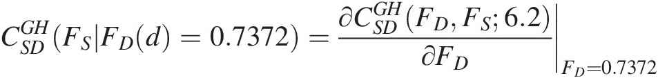
To be consistent with the discussion in Chapter 5, we assign the conditional copula as the h function:CSDGHFSFDd=0.7372=hGHFSFD6.2=0.7869
 . The conditional copula for the Gumbel–Hougaard copula is listed as No. 4 in Table 4.2. As seen in Table 4.2, U(2) needs to be solved for numerically using the root-finding (e.g., bisection method) technique. Using the bisection method, we have the following:
U(2) = FS(s) = h−1(0.7869, 0.7372; 6.2) = 0.777.U2=FSs=h−10.78690.73726.2=0.777.
3. Compute U(3)U3, i.e., FMDIFMDI:
From the vine structure, we have the following:
w3=C3∣12U3U1U2=∂C13∣2C23U3U2C12U1U2∂C12U1U2=∂D,MDI∣SGaussianCMDI,SFrankFMDIFSs11.47CS,DGHFDFSs6.2−0.418∂CS,DGHFDFSs6.2and U(3)U3 can then be computed with the following three steps: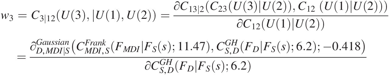
a. Compute the conditional copula CS,DGHFDFS
 . From the first two steps, we have FD = 0.7372, FS = 0.777FD=0.7372,FS=0.777; CS,DGHFSFD6.2
 can then be computed by substituting FD = 0.7372, FS = 0.777, θ = 6.2FD=0.7372,FS=0.777,θ=6.2 into No. 4 conditional copula in Table 4.2. We obtain the following:
CS,DGHFDFS6.2=C0.73720.7776.2=0.2791
b. Compute the conditional copula of CMDI,SFrankFMDIFSs11.47
 with the use of the meta-Gaussian copula fitted to T2 by setting the h function as follows:
w3=hgaussianCMDI,SFrankFMDIFS11.47CS,DGHFDFS6.2−0.418=0.6537and we have the following: CMDI,SFrankFMDIFS11.47=hgaussian−10.65370.2791−0.418

For the Gaussian copula, its conditional copula is the univariate normal distribution. The derivation of the conditional copula is given as Equation (7.42). In this particular problem, Equation (7.42a) can be rewritten as follows:
hgaussianCMDI,SFrankFMDIFS11.47CS,DGHFDFS6.2−0.418
~ΦΦ−1CMDI,SFrankFMDIFS11.47−ρΦ−1CS,DGHFDFS6.21−ρ20.5LethMDI,S=CMDI,SFrankFMDIFS11.47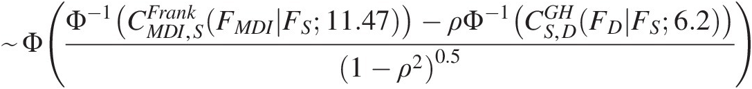
 we have:
Φ−1hMDI,S=Φ−1w31−ρ20.5+ρΦ−1(CS,DGHFDFSs6.2
and hMDI,S=CMDI,SFrankFMDIFS11.47=Φ0.571=0.716
=(1 − (−0.418)2)0.5Φ−1(0.6537) − 0.418Φ−1(0.2791) = 0.571=1−−0.41820.5Φ−10.6537−0.418Φ−10.2791=0.571 .
.
c. Compute FMDIFMDI from CMDI,SFrankFMDIFS11.47
 .
.
In steps b, we have computed CMDI,SFrankFMDIFS11.47=0.716
 . Using the conditional Frank copula in Table 4.2, we have the following:
U(3) = FMDI(mdi) = h−1(0.716, 0.777; 11.47) = 0.8421U3=FMDImdi=h−10.7160.77711.47=0.8421.


To this end, we have finished one simulation:
To repeat the preceding procedure, we can simulate the random variables of size N.
By applying the fitted marginal distributions we obtain the simulation in the real domain as follows:

Applying the linear interpolation of FMDIFMDI to [MDI, empirical distribution of MDI], we have the following:
MDIsimu = 1534.9 cfsMDIsimu=1534.9cfs. Finally, we have the corresponding simulation in the real domain as follows:

Figure 13.13 Comparison of observed drought variables with simulations from the fitted vine copula.
Figure 13.14 compares the sample Kendall’s tau of the observed trivariate drought variables with those computed using the simulated trivariate variables from the vine copula. Comparison shows that the dependence structure of the drought variables is well preserved. The fitted vine copula may be applied further for risk analysis.

Figure 13.14 Comparison of sample Kendall’s tau and those simulated from the fitted vine copula.
Joint and Conditional Return Period through Vine Copula
In this section, we will proceed with risk analysis through the joint and conditional return period. In the case of joint return period, we will only investigate the “AND” case.
Joint Return Period “AND” Case
Similar to the bivariate case, the trivariate return period of the “AND” case can be given as follows:
 (13.12)
where
 (13.12a)
To compute using Equation (13.12a), we will need to first evaluate CD, MDI(FD, FMDI)CD,MDIFDFMDI. CD, MDI(FD, FMDI)CD,MDIFDFMDI is the 2-margin of the trivariate copula as follows:
 (13.13)
where f(t) = 1ft=1 for the uniformly distributed random variable on [0, 1].
Figure 13.15 compares the empirical copula and that computed using Equation (13.13). In Figure 13.15, we also plot the joint CDF of D and MDI estimated separately using the Gumbel–Hougaard copula (θ = 2.22)θ=2.22). The goodness-of-fit study ensures the appropriateness with SnB = 0.05; Pvalue = 0.91SnB=0.05;Pvalue=0.91. From Figure 13.15, we see that there is minimal difference between the computed joint CDF (i.e., for D and DMI) using Equation (13.13) and that computed directly from the Gumbel–Hougaard copula (the maximum absolute difference is 0.028). To reduce the complexity of computation, we will directly apply the Gumbel–Hougaard copula to D and MDI. Setting MDI ≥ 1526.1 cfsMDI≥1526.1cfs (i.e., equivalent to FMDI(mdi ≤ 1526.1) = 0.8FMDImdi≤1526.1=0.8), Figures 13.16 and 13.17 plot the joint exceedance probability (i.e., equivalent to survival copula) and the corresponding joint return period. Table 13.15 lists the sample results for computing the exceedance joint probability and its joint return period. As shown in Figures 13.16 and 13.17, the exceedance probability shows the concave shape and the joint return period shows the convex shape with MDI ≥ 1.53E + 03 cfsMDI≥1.53E+03cfs as the example graphed. It shows the low exceedance probability and high return period for a long duration with low drought severity, as well as for the short duration with high drought severity. The moderate drought duration and drought severity yield a shorter return period than does high drought severity with a short duration. We should note that with the change of plotted examples for MDI (or D or S), the shape may change accordingly.


Figure 13.16 Exceedance probability for C(D ≥ d, S ≥ s, MDI ≥ 1.53E + 03cfs)CD≥dS≥sMDI≥1.53E+03cfs.

Table 13.15. Exceedance joint CDF and joint return period (“AND” case) with MDI ≥ 1.53E + 03 cfsMDI≥1.53E+03cfs.
| Frequency domain | FDFD | ||||||
|---|---|---|---|---|---|---|---|
| 0.2 | 0.5 | 0.9 | 0.95 | 0.99 | |||
| Exceed. joint CDF | FSFS | 0.2 | 0.199 | 0.192 | 0.078 | 0.042 | 0.009 |
| 0.5 | 0.199 | 0.192 | 0.078 | 0.042 | 0.009 | ||
| 0.9 | 0.136 | 0.170 | 0.078 | 0.042 | 0.009 | ||
| 0.95 | 0.109 | 0.156 | 0.077 | 0.041 | 0.009 | ||
| 0.99 | 0.084 | 0.142 | 0.074 | 0.040 | 0.009 | ||
| Real domain | D (days)a | ||||||
|---|---|---|---|---|---|---|---|
| 38 | 135 | 520 | 699 | 1133 | |||
| Joint return period (yrs) | S | 7860 | 3.626 | 3.774 | 9.281 | 17.402 | 83.468 |
| (cfs.day) | 26880 | 3.633 | 3.774 | 9.281 | 17.402 | 83.468 | |
| 174920 | 5.298 | 4.265 | 9.292 | 17.402 | 83.468 | ||
| 297460 | 6.620 | 4.634 | 9.424 | 17.424 | 83.468 | ||
| 805320 | 8.595 | 5.078 | 9.727 | 17.875 | 83.546 | ||
a The duration is rounded to the nearest integer number.
Conditional Return Period with the Constructed Vine Copula
Here we will investigate the following cases for the conditional return period as examples:
(i) D>d ∩ MDI>mdi ∣ S ≤ sD>d∩MDI>mdi∣S≤s
(ii) D>d ∩ MDI>mdi ∣ S = sD>d∩MDI>mdi∣S=s
(iii) D>d ∪ MDI>mdi ∣ S ≤ sD>d∪MDI>mdi∣S≤s
(iv) D>d ∪ MDI>mdi ∣ S = sD>d∪MDI>mdi∣S=s
(iv) D>d ∣ MDI ≤ mdi ∩ S ≤ sD>d∣MDI≤mdi∩S≤s
(vi) D>d ∣ MDI = mdi ∩ S = sD>d∣MDI=mdi∩S=s
Cases (i) and (ii): D>d ∩ MDI>mdi ∣ S ≤ SD>d∩MDI>mdi∣S≤S and D>d ∩ MDI>mdi ∣ S = sD>d∩MDI>mdi∣S=s
Cases (i) and (ii) investigate the impact of drought severity on drought duration and MDI during the drought episode under the condition of both D and MDI exceeding the corresponding critical level.
The conditional exceedance probability P(D>d ∩ MDI>mdi| S ≤ s)PD>d∩MDI>mdiS≤s for case (i) may be written as follows:
 (13.14)
and the corresponding conditional return period can simply be given as follows:
 (13.14a)
The conditional exceedance probability P(D>d ∩ MDI>mdi| S = s)PD>d∩MDI>mdiS=s may be written as follows:
 (13.15)
where
 (13.15a)
 (13.15b)
Applying FS = [0.2, 0.5, 0.9, 0.95, 0.99]FS=0.20.50.90.950.99 for the conditioning severity, we have the drought severity estimated as S≈[7860, 26880, 174920, 297460, 805320]S≈786026880174920297460805320cfs.day.
Table 13.16 lists and Figures 13.18 and 13.19 plot the conditional return period for cases (i) and (ii) using S = 174920 cfs.day as an example.
Table 13.16. Conditional exceedance probability and conditional return period: cases (i) and (ii).
| Case (i) | Case (ii) | |||||||
|---|---|---|---|---|---|---|---|---|
| MDI>mdiMDI>mdi (cfs) | MDI>mdiMDI>mdi (cfs) | |||||||
| 646 | 1106 | 1537 | 646 | 1106 | 1537 | |||
| Conditional exceedance prob. | D > d (day) | 38 | 0.573 | 0.295 | 0.005 | 1.00 | 1.00 | 0.45 |
| 135 | 0.295 | 0.131 | 0.001 | 0.99 | 0.99 | 0.44 | ||
| 520 | 0.023 | 0.007 | 1.84E−05 | 0.41 | 0.41 | 0.12 | ||
| 699 | 0.008 | 0.002 | 4.27E−06 | 0.20 | 0.20 | 0.043 | ||
| 1133 | 0.001 | 2.38E−04 | 2.46E−07 | 0.037 | 0.037 | 0.005 | ||
| Conditional return period | D > d (day) | 38 | 1.26 | 2.45 | 160.04 | 0.72 | 0.72 | 1.62 |
| 135 | 2.45 | 5.52 | 636.34 | 0.73 | 0.73 | 1.65 | ||
| 520 | 31.24 | 103.24 | 3.94E+04 | 1.78 | 1.78 | 6.22 | ||
| 699 | 85.11 | 316.69 | 1.69E+05 | 3.66 | 3.66 | 16.67 | ||
| 1133 | 658.89 | 3038.20 | 2.93E+06 | 19.45 | 19.46 | 151.40 | ||

Figure 13.18 Conditional exceedance probability and conditional return period: case (i).

Figure 13.19 Conditional exceedance probability and conditional return period: case (ii).
Cases (iii) and (iv): D>d ∪ MDI>mdi ∣ S ≤ s; D>d ∪ MDI>mdi ∣ S = SD>d∪MDI>mdi∣S≤s;D>d∪MDI>mdi∣S=S
Cases (iii) and (iv) again investigate the impact of drought severity on drought duration and MDI but under different conditions, i.e., at least one drought variable (D or MDI) exceeding the corresponding critical level.
The conditional exceedance probability P(D>d ∪ MDI>mdi| S>s)PD>d∪MDI>mdiS>s of case (iii) may be rewritten with the following set of equations as follows:
 (13.16)
The corresponding joint return period is then written as follows:
 (13.16a)
The conditional exceedance probability P(D>d ∪ MDI>mdi| S = s)PD>d∪MDI>mdiS=s of case (iv) can be written as follows:
 (13.17)
Here it is obvious that CD, MDI ∣ SCD,MDI∣S in Equation (13.17) is nothing but the copula function at T2 of the vine structure. The corresponding conditional return period can be written as follows:
 (13.17a)
Figures 13.20 and 13.21 plot the conditional exceedance probability and the conditional return period for cases (iii) and (iv) using S = 174920 cfs.day as an illustrative sample. Table 13.17 lists the sample results.

Figure 13.20 Conditional exceedance probability and the corresponding conditional joint return period for case (iii).

Figure 13.21 Conditional exceedance probability and corresponding conditional joint return period for case (iv).
Table 13.17. Conditional exceedance probability and conditional return period: cases (iii) and (iv).
| Case (iii) | Case (iv) | |||||||
|---|---|---|---|---|---|---|---|---|
| MDI>mdiMDI>mdi (cfs) | MDI>mdiMDI>mdi (cfs) | |||||||
| 646 | 1106 | 1537 | 646 | 1106 | 1537 | |||
| Conditional exceedance prob. | D > d (day) | 38 | 0.98 | 0.93 | 0.79 | 1.00 | 1.00 | 1.00 |
| 135 | 0.93 | 0.76 | 0.46 | 1.00 | 1.00 | 1.00 | ||
| 520 | 0.81 | 0.49 | 0.06 | 1.00 | 1.00 | 0.74 | ||
| 699 | 0.79 | 0.46 | 0.03 | 1.00 | 1.00 | 0.60 | ||
| 1,133 | 0.78 | 0.45 | 0.02 | 1.00 | 1.00 | 0.48 | ||
| Conditional return period | D > d (day) | 38 | 0.74 | 0.78 | 0.92 | 0.72 | 0.72 | 0.72 |
| 135 | 0.78 | 0.95 | 1.58 | 0.72 | 0.72 | 0.72 | ||
| 520 | 0.90 | 1.48 | 11.52 | 0.72 | 0.72 | 0.98 | ||
| 699 | 0.91 | 1.56 | 21.46 | 0.72 | 0.72 | 1.20 | ||
| 1,133 | 0.93 | 1.61 | 45.04 | 0.72 | 0.72 | 1.51 | ||
Cases (v) and (vi): D>d ∣ MDI ≤ mdi ∩ S ≤ sD>d∣MDI≤mdi∩S≤s and D>d ∣ MDI = mdi ∩ S = sD>d∣MDI=mdi∩S=s
Cases (v) and (vi) investigate the combined impact of maximum drought intensity and severity on drought duration.
For case (v), its conditional exceedance probability may be written as follows:
 (13.18)
and the corresponding conditional joint return period can be written as follows:
 (13.18a)
For case (VI), its conditional exceedance probability can be written as follows:
 (13.19)
The corresponding conditional return period may be estimated through the vine copula as follows:
 (13.19a)
The copula functions in Equation (13.19) directly reflect the constructed vine copula, i.e., CMDI, D ∣ SCMDI,D∣S is Gaussian copula of T2, and CD, SCD,S and CMDI, SCMDI,S are the Gumbel–Hougaard and Frank copula of T1.
Table 13.18 lists the sample results using [S = 174920 cfs.day, MDI = 1526 cfs], [S = 25000 cfs.day, MDI = 800 cfs], and [S = 10000 cfs.day, MDI = 1000 cfs] as the illustration samples. Figures 13.22 and 13.23 plot the conditional exceedance probability and the corresponding conditional return period for cases (v) and (vi).
Table 13.18. Sample results for cases (v) and (vi).
| Case (v) | Case (vi) | |||||||
|---|---|---|---|---|---|---|---|---|
| S ≤ s (cfs. day); MDI ≤ mdiS≤scfs.day;MDI≤mdi (cfs) | S = s; MDI = mdiS=s;MDI=mdi | |||||||
| S = 174920; MDI = 1526 | S = 25000; MDI = 800 | S = 10000; MDI = 1000 | S = 174920; MDI = 1526 | S = 25000; MDI = 800 | S = 10000; MDI = 1000 | |||
| Conditional exceedance prob. | D > d (day) | 38 | 0.81 | 0.68 | 0.28 | 1.00 | 1.00 | 0.60 |
| 135 | 0.48 | 0.09 | 3.16E-03 | 1.00 | 0.58 | 0.002 | ||
| 520 | 0.01 | 1.07E-06 | 2.68E-08 | 0.56 | 6.99E-06 | 3.80E-10 | ||
| 699 | 2.24E-04 | 1.24E-08 | 3.09E-10 | 0.01 | 5.14E-08 | 1.18E-12 | ||
| 1133 | 9.16E-09 | 5.04E-13 | 1.26E-14 | 1.40E-07 | 6.09E-13 | 0 | ||
| Conditional return period | D > d (day) | 38 | 0.89 | 1.06 | 2.59 | 0.72 | 0.72 | 1.21 |
| 135 | 1.50 | 8.19 | 229.10 | 0.72 | 1.24 | 369.24 | ||
| 520 | 51.20 | 6.75E+05 | 2.69E+07 | 1.29 | 1.03E+05 | 1.90E+09 | ||
| 699 | 3234.94 | 5.85E+07 | 2.34E+09 | 63.30 | 1.41E+07 | 6.12E+11 | ||
| 1133 | 7.89E+07 | 1.43E+12 | 5.74E+13 | 5.16E+06 | 1.19E+12 | Inf | ||

Figure 13.22 Conditional exceedance probability and conditional return period: case (v).

Figure 13.23 Conditional exceedance probability and conditional return period: case (vi).
Elliptical-Copula Approach to Model Trivariate Drought Variables
In this section, we apply the elliptical copula to model the trivariate drought variables as well as evaluate the corresponding risk through return period. Not to complicate the process, the Gaussian and Student t copulas are adopted for analysis. Applying MLE, Table 13.19 lists the parameters estimated from both the copulas with the use of empirical marginals. From this point on, we will use the Student t copula as an example to illustrate the application. Figures 13.24 and 13.25 compare the simulated variables with the observed variables in both frequency and real domains. Figure 13.24 indicates a good comparison between pseudo-observations and simulations. In Figure 13.25 (real domain comparison), the comparison does not look as good as that in Figure 13.24 due to the ties in drought variables: D and DMI.
Table 13.19. Parameters estimated for elliptical copulas.
| Gaussian | T | |||||
|---|---|---|---|---|---|---|
| S | D | DMI | S | D | DMI | |
| S | 1 | 0.95 | 0.87 | 1 | 0.96 | 0.87 |
| D | 0.95 | 1 | 0.76 | 0.96 | 1 | 0.78 |
| DMI | 0.87 | 0.76 | 1 | 0.87 | 0.78 | 1 |
| ν = 19.14ν=19.14 | ||||||

Figure 13.24 Comparison of simulated random variables with the pseudo-observations.

Figure 13.25 Comparison of simulated drought variables with observed drought variables.
Joint and Conditional Return Period from the Student T Copula
With the chosen Student t copula, we will again evaluate the joint return period (“AND”) and all six cases of the conditional return period that are applied to the vine copula.
Joint Return Period (“AND”) Case
As shown previously, we will need to apply Equation (13.13), in which the bivariate copula margins are as follows: C(FS, FD) = C(FS, FD, 1); C(FS, FMDI) = C(FS, 1, FMDI); C(FD, FMDI) = C(1, FS, FMDI)CFSFD=CFSFD1;CFSFMDI=CFS1FMDI;CFDFMDI=C1FSFMDI. In the case of Student t copula, the two margins are also bivariate copulas with the degree of freedom being the same as that of multivariate student t copula. As an example, C(FS, FD)CFSFD is a bivariate strudent copula with Σ=10.960.961,ν=19.14 . Applying Equation (13.13), Figure 13.26 plots the joint exceedance probability and the corresponding joint return period. As before, we set FMDI = 0.8FMDI=0.8 as an illustrative example. Table 13.20 lists the sample results.
Table 13.20. Sample results of the joint return period computed from the Student t copula.
| Frequency domain | FDFD | ||||||
|---|---|---|---|---|---|---|---|
| 0.2 | 0.5 | 0.9 | 0.95 | 0.99 | |||
| Exceed. joint CDF | FSFS | 0.2 | 0.199 | 0.187 | 0.078 | 0.043 | 0.010 |
| 0.5 | 0.196 | 0.187 | 0.078 | 0.043 | 0.010 | ||
| 0.9 | 0.088 | 0.088 | 0.070 | 0.043 | 0.010 | ||
| 0.95 | 0.048 | 0.048 | 0.046 | 0.037 | 0.010 | ||
| 0.99 | 0.010 | 0.010 | 0.010 | 0.010 | 0.007 | ||
| Real domain | D (days)[1] | ||||||
|---|---|---|---|---|---|---|---|
| 38 | 135 | 520 | 699 | 1133 | |||
| Joint return period (yrs) | S | 7860 | 3.63 | 3.87 | 9.33 | 16.65 | 75.10 |
| (cfs.day) | 26880 | 3.69 | 3.87 | 9.33 | 16.65 | 75.10 | |
| 174920 | 8.20 | 8.20 | 10.30 | 16.85 | 75.10 | ||
| 297460 | 15.14 | 15.14 | 15.78 | 19.77 | 75.25 | ||
| 805320 | 72.66 | 72.66 | 72.68 | 73.09 | 101.74 | ||

Figure 13.26 Plot of joint exceedance probability and the corresponding return period.
Conditional Return Period Estimated Using the Student t Copula
Rather than considering all six cases as those for the Vine copula approach, here we will only investigate the following three cases:
1. Case: D>d ∩ MDI>mdi ∣ S ≤ sD>d∩MDI>mdi∣S≤s
Identical to the vine copula approach discussed earlier, the survival copula and the two margins need to be assessed, so as to evaluate the conditional return period. As shown in the joint return period “AND” case, the two margins of the Student t copula can be easily computed. Applying Equation (13.13) and using S = 174920 cfs.day as an example, Table 13.21 lists the sample results. Figure 13.27 provides the sample plots for conditional exceedance probability and conditional return period.
2. Case: D>d ∪ MDI>mdi ∣ S ≤ sD>d∪MDI>mdi∣S≤s
Equation (13.15) is applied to compute the conditional exceedance probability and conditional return period. Using S = 174290 cfs.day as an example, Table 13.22 lists the sample results. Figure 13.28 provides sample plots.
3. Case: MDI>mdi ∣ D ≤ d ∩ S ≤ sMDI>mdi∣D≤d∩S≤s
Equation (13.17) (i.e., the general form) is applied to compute the conditional exceedance probability and conditional return period for this case. Table 13.23 lists sample results. Figure 13.29 provides sample plots.
Table 13.21. Conditional exceedance probability and conditional return periods: D>d ∩ MDI>mdi ∣ S ≤ sD>d∩MDI>mdi∣S≤s.
| MDI>mdiMDI>mdi (cfs) | |||||
|---|---|---|---|---|---|
| 646 | 1106 | 1537 | |||
| Conditional exceedance prob. | D > d (day) | 38 | 0.696 | 0.430 | 0.022 |
| 135 | 0.430 | 0.325 | 0.019 | ||
| 520 | 0.038 | 0.035 | 0.002 | ||
| 699 | 0.010 | 0.009 | 0.001 | ||
| 1,133 | 3.01E-04 | 2.69E-04 | 9.92E-06 | ||
| Conditional return period | D > d (day) | 38 | 1.04 | 1.68 | 32.93 |
| 135 | 1.68 | 2.22 | 37.10 | ||
| 520 | 19.12 | 20.75 | 301.30 | ||
| 699 | 74.15 | 79.86 | 1,387.011 | ||
| 1,133 | 2.41E+03 | 2.69E+03 | 7.29E+04 | ||

Figure 13.27 Conditional exceedance probability and conditional return period: D>d ∩ MDI>mdi ∣ S ≤ sD>d∩MDI>mdi∣S≤s.
Table 13.22. Conditional exceedance probability and conditional return periods: D>d ∪ MDI>mdi ∣ S ≤ sD>d∪MDI>mdi∣S≤s.
| MDI>mdiMDI>mdi (cfs) | |||||
| 646 | 1106 | 1537 | |||
| Conditional exceedance prob. | D > d (day) | 38 | 0.860 | 0.792 | 0.778 |
| 135 | 0.792 | 0.564 | 0.448 | ||
| 520 | 0.778 | 0.448 | 0.058 | ||
| 699 | 0.778 | 0.445 | 0.031 | ||
| 1,133 | 0.778 | 0.444 | 0.022 | ||
| Conditional return period | D > d (day) | 38 | 0.84 | 0.91 | 0.93 |
| 135 | 0.91 | 1.28 | 1.62 | ||
| 520 | 0.93 | 1.62 | 12.52 | ||
| 699 | 0.93 | 1.62 | 23.02 | ||
| 1,133 | 0.93 | 1.63 | 32.24 | ||

Figure 13.28 Conditional exceedance probability and conditional return period: D>d ∪ MDI>mdi ∣ S ≤ sD>d∪MDI>mdi∣S≤s.
Table 13.23. Conditional exceedance probability and conditional return periods: D>d ∣ MDI ≤ mdi ∩ S ≤ sD>d∣MDI≤mdi∩S≤s.
| Case (v) | |||||
|---|---|---|---|---|---|
| S ≤ s (cfs. day); MDI ≤ mdiS≤scfs.day;MDI≤mdi (cfs) | |||||
| S = 174920; MDI = 1526 | S = 25000; MDI = 800 | S = 10000; MDI = 1000 | |||
| Conditional exceedance prob. | D > d (day) | 38 | 0.75 | 0.46 | 0.26 |
| 135 | 0.38 | 0.06 | 2.56E-03 | ||
| 520 | 0.02 | 6.26E-06 | 8.10E-08 | ||
| 699 | 1.83E-03 | 2.86E-07 | 5.50E-09 | ||
| 1,133 | 4.33E-06 | 1.24E-09 | 5.13E-11 | ||
| Conditional return period | D > d (day) | 38 | 0.97 | 1.56 | 2.80 |
| 135 | 1.89 | 1.16E+01 | 2.83E+02 | ||
| 520 | 45.14 | 1.15E+05 | 8.92E+06 | ||
| 699 | 3.95E+02 | 2.52E+06 | 1.32E+08 | ||
| 1,133 | 1.67E+05 | 5.85E+08 | 1.41E+10 | ||

Figure 13.29 Conditional exceedance probability and conditional return period: D>d ∣ MDI ≤ mdi ∩ S ≤ sD>d∣MDI≤mdi∩S≤s.
13.3.5 Comparison of Vine Copula and Student T Copula for Trivariate Drought Analysis
In this section, we will further compare the differences yielded from the fitted vine copula and simple trivariate Student t copula by (1) overall performance through the joint CDF; (2) joint return period of the “AND” case; and (iii) six cases of the conditional return period.
Overall Performance through Joint CDF
To compare the overall difference, Figure 13.30 compares the empirical CDF with the joint CDF computed from the fitted GH–Frank–Gaussian vine and Student t copulas. As shown in Figure 13.30, the overall performance is very similar to the fitted Student t copula and vine copula. Figure 13.30 indicates the possible underestimation of the joint probability for higher drought severity, duration, and MDI from both fitted vine and Student t copulas. The RMSE is computed as 0.019 and 0.017 for the fitted vine and Student t copulas, respectively, which further explains their similar overall performance.

Joint Return Period “AND” Case
Tables 13.15 and 13.20 list the sample results for the joint return period “AND” case computed from the fitted vine copula and Student t copula, respectively. Figures 13.16(a), 13.17(a), and 13.26 provide the sample plot for the joint return period “AND” case. MDI = 1.53E03MDI=1.53E03 cfs (i.e., FMDI(MDI ≤ 1.53E03 cfs) = 0.8FMDIMDI≤1.53E03cfs=0.8) is applied for the table results and sample plots. Results show similar joint return periods (i.e., the risk of D, S, and MDI all exceeding the critical threshold). Let us consider the univariate D and S with nonexceedance probability of 0.99 as an example. As discussed earlier in Section 13.3.2, we have DF(d) = 0.99 = 1133 day, SF(s) = 0.99 = 805320 cfs. dayDFd=0.99=1133day,SFs=0.99=805320cfs.day using the Weibull and log-normal distributions fitted to D and S. From the fitted vine copula and Student t copula, we obtain the following:
Vine copula: T(D ≥ 1133 day ∩ S>805320 cfs. day ∩ MDI>1530 cfs)≈83.5TD≥1133day∩S>805320cfs.day∩MDI>1530cfs≈83.5yrs.
Student t copula: T(D ≥ 1133 day ∩ S>805320 cfs. day ∩ MDI>1530 cfs)≈TD≥1133day∩S>805320cfs.day∩MDI>1530cfs≈102 yrs.
It is seen that the vine copula yields a smaller return period (i.e., higher risk) for all three drought variables exceeding the threshold values compared to the Student t copula. It is partly due to the negative correlation of T2 (ρ≈ − 0.42)ρ≈−0.42) for the fitted Gaussian copula at T2, while the positive variance-covariance structure is shown for Student t copula (Table 13.19). Both vine and Student t copulas show that it is more realistic to study the dependence than assuming that the variables are independent. With the assumption of the independence, we will have Tand = EINT/(1 − FS)(1 − FD)(1 − FMDI)Tand=EINT/1−FS1−FD1−FMDI, and substituting EINT = 0.73, FS = 0.99, FD = 0.99, FMDI = 0.8EINT=0.73,FS=0.99,FD=0.99,FMDI=0.8, we get Tand≈36500 yrTand≈36500yr.
In one aspect, considering the fitted GH–Frank–Gaussian vine copula for drought variables D, S, and MDI, we have Gumbel–Hougaard, Frank, and Gaussian copulas applied to model {D, S}, {S, MDI}, and {D|S, MDI|S}, respectively. This is done, purely based on the dependence (i.e., degree of association) among drought variables. Compared to the sample rank-based Kendall correlations among all three drought variables, the drought severity has higher dependence on drought duration (0.83) and MDI (0.71). As the result, S is set as the center variable as shown in the section “Vine-Copula Approach to Model Trivariate Drought Variables.” In addition, to estimate the joint exceedance probability and the corresponding joint return period “AND” case, we will need to estimate the copula (i.e., JCDF) for {D, MDI}. The copula of {D, MDI} is also called 2-margins of the trivariate copula. Since {D, MDI} is not directly linked with the fitted vine copula, the numerical integration is involved (i.e., Equation (13.13)). The numerical integration may further accumulate the computational error (or may also be called computational uncertainty).
In the other aspect, belonging to the meta-elliptical copula family, the Student t copula is constructed upon the correlation matrix directly. As the result, it is not needed to rearrange the variables, while rearranging variables is a common case for the vine copula. In addition, the two margins of the multivariate Student t copula are the bivariate Student t copula with the same degree of freedom as that of multivariate Student t copula. In the case of computing the joint exceedance probability (and joint return period “AND” case), its computation is simpler than that for the fitted vine copula.
Conditional Return Period of Cases (i), (iii), and (v)
Cases (i): D>d ∩ MDI>mdi ∣ S ≤ sD>d∩MDI>mdi∣S≤s
As discussed in the previous sections, case (i) investigates the risk of both D and MDI exceeding the given thresholds with S smaller than the given threshold. For this case, the conditional return periods obtained from the vine copula are generally higher than those obtained from the Student t copula, which means the risk of exceedance is lower from the vine copula than that from the Student t copula.
Cases (iii): D>d ∪ MDI>mdi ∣ S ≤ sD>d∪MDI>mdi∣S≤s
Case (iii) investigates the risk of at least one of D or MDI exceeding the given threshold with S smaller than its given threshold. As expected, the risk is higher for at least one of D or MDI exceeding the given threshold from cases (iii) than that from cases (i). For example, with D>DF(d) = 0.99 ∪ MDI>MDIF(mdi) = 0.1 ∣ S ≤ SF(s) = 0.8D>DFd=0.99∪MDI>MDIFmdi=0.1∣S≤SFs=0.8, we compute the return period as about 45 and 32 years from the vine and Student t copulas for case (iii). The corresponding risk obtained from the Student t copula is higher than that from the vine copula.
Cases (v): D>d ∣ MDI ≤ mdi ∩ S ≤ sD>d∣MDI≤mdi∩S≤s
Case (v) investigates the risk of D exceedance under the condition of both MDI and S smaller than their threshold. Different from cases (i) and (iii), the return period reduces to the univariate case under the given condition for cases (v). The sample results in the table indicate a high risk for D to exceed a lower threshold value. With the increase of MDI and S, the risk is significantly reduced for D to exceed a higher threshold value.
13.4 Summary
In this chapter, we apply the copula theory to drought frequency analysis, including bivariate and trivariate cases. For the bivariate drought frequency analysis (drought duration and drought severity), the Archimedean and meta-elliptical (Gaussian and Student t) copulas are applied. For trivariate drought frequency analysis (drought duration, drought severity, and MDI of the drought event), the vine and meta-elliptical copulas are applied. The bivariate Archimedean and meta-elliptical copulas are applied as the candidates to construct the vine copula. Throughout this case study, we reach the following conclusions:
1. Similar to many other investigations, the log-normal and Weibull distributions are fitted to drought severity and drought duration, respectively. Due to the difficulty to fit a proper distribution directly to the MDI, the nonlinear meta-Gaussian transformation is applied to model the MDI such that standard Gaussian distribution may be applied to model the transformed variable
2. The Gumbel–Hougaard copula is most proper to model drought severity and drought duration. Conceptually, it is understandable for the applicability of this particular copula: (i) the GH copula belongs to the extreme value family, which may better represent the extremes in the nature of drought events; and (ii) the upper-tail dependence of the GH copula may better evaluate the risk of S>s|D>d (or S>s|D=d) and vice versa.
3. The dynamic return period may be assessed for the evolution of a certain drought episode. The case example shows that as the drought episode evolves, the dynamic return period goes up and down as well.
4. Both vine and Student t copulas are applied to model the trivariate drought variables. Compared to the vine copula, the Student t copula may be easier to apply with less computational burden to study risk. In addition, the design based on the risk computed from the Student t copula could be more conservative, since for a given condition, the risk from the Student t copula (lower return period) is generally higher than that from the vine copula (higher return period).
5. Similar to other investigations, the case study presented here assumes all drought variables as continuous random variables. However, for daily (or monthly) values, the duration is actually discrete and may be with many ties (i.e., one duration may be associated with at least two different drought severities). Compared to the commonly applied drought analysis with the use of monthly values, the analysis with daily values significantly cuts down the ties existing within the dataset. It may be worth the effort to actually try to model the duration as discrete variables.