Abstract
Air pollutants may be transferred via dry and wet deposition to other media such as soil, surface waters, vegetation, and buildings. These pollutants may then contaminate these surfaces and have adverse impacts on ecosystems, vegetation, and the built environment. In addition, some chemical species that do not have any adverse health effects via inhalation may become toxic via bioaccumulation in the food chain and subsequent ingestion. This chapter describes briefly the impacts of air pollutant deposition on ecosystems, agricultural crops, and buildings, as well as the indirect adverse effects on human health via the food chain.
Air pollutants may be transferred via dry and wet deposition to other media such as soil, surface waters, vegetation, and buildings. These pollutants may then contaminate these surfaces and have adverse impacts on ecosystems, vegetation, and the built environment. In addition, some chemical species that do not have any adverse health effects via inhalation may become toxic via bioaccumulation in the food chain and subsequent ingestion. This chapter describes briefly the impacts of air pollutant deposition on ecosystems, agricultural crops, and buildings, as well as the indirect adverse effects on human health via the food chain.
13.1 Ozone
Ozone is an air pollutant that has adverse health effects on humans (see Chapter 12). It also has adverse impacts on vegetation (EPA, 2007). These effects may be significant on crop yields and, therefore, may translate into economic impacts due to reduced agricultural crop production. Ozone may also show impacts on forests, as is the case, for example, in California.
The first symptoms of ozone deposition on vegetation appear on the outer layer of leaves. They are more important on leaves that are exposed to sunlight. The effects vary depending on the type of vegetation (e.g., deciduous trees, conifers, agricultural crops). The main symptoms are a discoloration of the leaves exposed to sunlight (photobleaching), small spots on the leaf surface (stippling and molting), and/or a brownish coloration on the upper parts of the leaves (bronzing). The mechanism leading to those symptoms may be summarized as follows. Ozone is absorbed by the plant stomata and reacts with organic molecules, such as isoprene and ethylene, which are present in the extracellular plant fluid. Oxidizing organic compounds are formed, which react with the proteins of the cellular membrane of the plant. This deterioration of the membrane leads to the visible effects corresponding to the exposure of the vegetation to high atmospheric ozone concentrations. Some other secondary effects also occur, such as a reduction in CO2 fixation (either via a perturbation of the enzymatic function or via stomata damage). The perturbation of the photosynthesis of the plant leads to accelerated aging of the leaves and a decrease in the root/shoot ratio and grain/biomass ratio. Therefore, there is a decrease in the grain yield and number of healthy leaves.
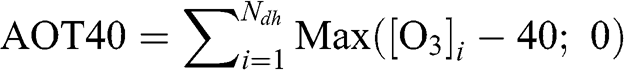
Exposure of vegetation to ozone must be quantified with a function that represents exposure above harmful levels. To that end, the AOT40 function (Accumulated ozone exposure over a threshold of 40 ppb) has been widely applied. The calculation of AOT40 is generally limited to daylight hours (solar radiation >50 W m−2). It corresponds to the cumulative exposure of vegetation to ozone concentrations greater than 40 ppb during daylight hours over a three-month period (from May to July) for agricultural crops and over a six-month period (April to September) for trees:
 (13.1)
 where Ndh represents the total number of daylight hours during the period of interest and [O3] is expressed in ppb. For example, the European Union has a target value of 3,000 ppb h for crops based on an AOT40 calculated using a daylight-hour period of 8 am to 8 pm Central European Time. Other exposure threshold values may be used. For example, a threshold value of 60 ppb is used in the SUM60 function. It is calculated in the same way as AOT40, but with an ozone concentration threshold of 60 ppb. The U.S. EPA currently uses a sigmoidal cumulative function, W126, which does not use an adverse exposure concentration threshold, but instead gives more weight to the higher concentrations. It is calculated for daylight hours between 8 am and 8 pm, i.e., for a twelve-hour period, as follows:
 (13.2)
 Next, the function is calculated over a three-month period:
 (13.3)
 where Nw is the total number of days during the three-month period (i.e., Nw = 91 or 92). (Adjustments are made for periods with missing O3 data.) W126 is calculated as a moving three-month average between April and October and the maximum value of the three-month averaged W126 is selected. Next, the average of these maximum values is calculated over a three-year period. The U.S. EPA currently uses W126 to estimate vegetation exposure to ozone and a range of 13,000 to 17,000 ppb h is considered acceptable to protect vegetation from ozone damage. Although there is no direct relationship between the U.S. health-based air quality standard (a concentration of 0.070 ppm averaged over 8 hours, referred to as the primary ambient air quality standard) and W126, the U.S. EPA considers that the primary standard should be protective of vegetation and has not proposed a secondary standard that would be specific to vegetation exposure.
The adverse effects of ozone on vegetation depend on the types of crops and trees, as some species are more resistant than others. Nevertheless, the impact of ozone on vegetation translates into significant economic impacts for agriculture. For example, ozone levels for the year 2000 have been estimated to lead to decreases in global crop yields ranging from 2 to 15 % depending on crop type (soybean, wheat or maize) and the methodology used (Avnery et al., 2011).
13.2 Acid Rain
The acidity of water is represented on a logarithmic scale by the pH. It is the negative value of the base 10 logarithm of the activity of the proton H+ (for a dilute solution, the activity is equivalent to the concentration; see Chapter 10):
Pure water has a neutral pH of 7 at 25 °C, since H+ and OH− are present in identical concentrations. However, liquid water in the atmosphere does not have a neutral pH, even in a pristine atmosphere. Carbon dioxide (CO2), which is naturally present in the atmosphere, is a weak acid, which is soluble in water. For an atmospheric CO2 concentration of 400 ppm (parts per million), the pH of a cloud droplet or raindrop is calculated to be 5.6 (see Chapter 10). Therefore, acid rain has a pH that is less than 5.6.
Chemical species that lead to acid rain are strong acids, i.e., they dissociate quasi totally in water into H+ and anions. In the atmosphere, the main strong acids are sulfuric acid (H2SO4), nitric acid (HNO3), and hydrochloric acid (HCl). The discovery of acid rain goes back to the beginning of the industrial era. Although the original references given in the English literature list mostly the work of R.A. Smith (1852, 1872), the first scientific article on that topic was published by a French pharmacist, M. Ducros (1845), who proposed that the acidity of the rain was due to nitric acid, resulting, for example, from the formation of nitrogen oxides during thunderstorms. A reanalysis of the data obtained by Smith on precipitation in the region of Manchester suggested that acidity was mostly due to HCl. It is possible that coal combustion in that region led to high atmospheric concentrations of HCl (chlorine is one of the compounds present in coal and it is emitted mostly as HCl during coal combustion).
One should note that acid rain is generally used as a term that covers more generally both wet and dry deposition. Wet deposition includes scavenging by rain, but also by snow and hail, as well as occult wet deposition (from mountain clouds and fogs). Dry deposition affects both particles (which may contain sulfate and nitrate) and gases (such as nitric acid); see Chapter 11. Therefore, the correct scientific term is “acid deposition,” rather than “acid rain.”
In the 1970s, regions such as Scandinavia in Europe and Canada in North America showed significant modifications in their lakes with significant decreases in their fish population. In addition, some forests such as the Black Forest in Germany showed important signs of decline. An analysis of the causes of these environmental changes showed that the pH of lakes had decreased significantly (i.e., lake acidification). In the forests, the rain acidity led to a change in the geochemistry with a modification of the chemical equilibria of the various inorganic chemical species (e.g., Reuss and Johnson, 1986). In particular, species such as magnesium (Mg) and calcium (Ca), which are nutrients for vegetation, became soluble ions. Thus, they were washed out by the rain and were no longer available for absorption by the roots of the trees. In addition, some elements that are toxic to vegetation, such as aluminum (Al), became available for absorption by roots. As a result, these different factors led to the death of a large number of trees in some regions. The main acids responsible for the acidification of lakes and soils were identified to be sulfuric acid and nitric acid.
These two acids are not emitted in the atmosphere in significant amounts, but are formed in the atmosphere by the chemical oxidation of primary pollutants emitted in the atmosphere (see Chapters 8 and 10):
Therefore, sulfuric acid and nitric acid are secondary pollutants.
Sulfur is present in coal, oil, and various minerals. Therefore, it is emitted during the combustion of coal (power plants, residential heating …), oil-derived fuels (diesel, gasoline …), and some industrial activities (smelters …), mostly in the form of sulfur dioxide (SO2). Nitrogen oxides (nitric oxide, NO, and nitrogen dioxide, NO2) are emitted during all combustion processes because nitrogen (N2) and oxygen (O2) present in the air react at the high temperatures of the combustion process to form these nitrogen oxides (mostly NO; NOx is used to represent the sum of NO and NO2). Since it takes some time for those primary pollutants to be oxidized into acids, acid rain pollution tends to cover long distances (several hundreds of kilometers). In addition, there are some natural sources of SO2 and NOx. Volcanic eruptions lead to significant emissions of SO2. Oceans emit dimethyl sulfide (DMS), which gets oxidized slowly into SO2. Soils emit nitrogen oxides (NOx, as well as nitrous oxide, N2O, a greenhouse gas). Lightning produces NOx in the high atmospheric layers (as suggested by Ducros, 1845). Table 2.1 summarizes the main categories of SO2 and NOx sources (see Chapter 2).
Another effect of acid rain is the degradation of buildings and statues (Brimblecombe, 2003). Some stones are calcareous (i.e., calcite, some marbles, freestone …). This calcareous compound is calcium carbonate, which reacts, for example, with sulfuric acid to lead to calcium sulfate (gypsum). This reaction leads to a change in the stone cohesiveness; the stone is no longer homogeneous in its chemical composition and some erosion of the stone occurs.
Acid deposition simulations are performed with three-dimensional (3D) atmospheric chemical-transport models. Such models were initially developed during the 1980s. The chemistry of the oxidation of SO2 into sulfuric acid and of NOx into nitric acid is rather well known (see Chapters 8 and 10). Figure 13.1 shows a comparison between wet deposition fluxes (precipitation) of simulated and measured sulfate at different stations of the National Acid Deposition Program (NADP) monitoring network in the United States. The spatial correlation between the simulation and measurements is satisfactory (determination coefficient of 0.77) and the model bias is low (8 %).

Figure 13.1. Comparison of simulated and measured wet deposition fluxes of sulfate in the United States for the year 1996.
SO2 and NOx emissions have been regulated in the 1980s in order to reduce acid deposition. For example, in the United States, SO2 and NOx emission regulations have been promulgated using a cap-and-trade approach (see Chapter 15). At the international level, the Göteborg protocol was introduced in 1999. It is officially called the “Gothenburg Protocol to Abate Acidification, Eutrophication and Ground-level Ozone”; therefore, it is also known as the “Multi-effect Protocol,” because it addresses several forms of air pollution (see Chapter 15). As of August 2017, 25 countries (including the U.S.) and the European Union had ratified this protocol, which defines ceiling targets for national emissions that must be attained by a given date (currently 2020). SO2 regulations have targeted mostly coal-fired power plants, smelters, and the sulfur content of gasoline and diesel fuels. NOx regulations have been mostly driven by the contribution of NOx species to ozone formation. Regulations have targeted emissions from on-road traffic, refineries, and fossil-fuel fired power plants. Long-term monitoring of sulfate and nitrate, as well as rain pH, has shown that these regulations were efficient and led to a decrease in acid deposition downwind of those sources. Most of the lakes and soils have seen their pH increase. However, some ecosystems recover faster than others, depending on their physico-chemical characteristics, and some lakes and forests are still under recovery. Nevertheless, it appears that overall the public policies introduced to reduce SO2 and NOx emissions have been effective in North America and in Europe, so that ecosystems that were adversely impacted in the 1970s are recovering and, in some cases, have recovered to their pre-industrial status. However, the acid deposition problem may now be present in some regions of Asia due to a fast industrial growth over the past several years.
13.3 Eutrophication
Vegetation needs nitrogen to grow. Plants obtain nitrogen naturally from the atmosphere and the soil. Agriculture uses nitrogenous fertilizers (for example, ammonium nitrate) to increase the yields of some crops. An increase in nitrogenous compound concentrations in water bodies leads, therefore, to an increase in aquatic vegetation. This increase in vegetation at the surface of the water body leads to a decrease in the amount of sunlight reaching the lower layers of the water body. This decrease in the solar radiation flux has a negative impact on plant photosynthesis (which converts carbon dioxide to oxygen) and the lower production of oxygen by plants leads to anoxic conditions (i.e., lack of oxygen). As a result, the concentrations of living organisms (e.g., phytoplankton, zooplankton) decrease, because of a lack of oxygen in the lower layers of the river, lake or sea. This phenomenon is called eutrophication. Its consequences are an increase in plants at the surface of the water body and a decrease in the aquatic life in the deep layers of that water body (e.g., Carpenter et al., 1998).
The main cause of eutrophication for most water bodies is the input of phosphorus and nitrogen originating from land-based human activities (e.g., use of fertilizers). Nevertheless, atmospheric deposition of nitrogen species contributes also to eutrophication (e.g., Bergström and Jansson, 2006). The main contributors to nitrogenous atmospheric deposition are nitric acid (which is also a contributor to acid deposition) and ammonia. Nitrogen oxides, NOx, are not very soluble in water and have low contributions to the dry and wet deposition fluxes of nitrogen overall. The contribution of organic nitrates is estimated to be commensurate to that of NOx and is, therefore, significantly less than those of nitric acid and ammonia (e.g., Vijayaraghavan et al., 2010). Anthropogenic sources of precursors (NOx) of nitric acid have been mentioned in Section 13.2. The main sources of atmospheric ammonia are agriculture-related activities: (1) the use of fertilizers for crops and (2) farm animals (cattle, pigs …). Table 2.1 summarizes the main source categories for nitrogen oxides and ammonia (see Chapter 2). The emissions of those pollutants are mostly regulated because of their air pollutant status in the case of NO2 and their role as precursors of ozone (NOx), acid deposition (NOx), and secondary fine particulate matter (NOx and NH3). Therefore, they are typically not targeted because of their eutrophication impacts. Nevertheless, this aspect is mentioned in some regulations, such as the Göteborg Protocol, which defines emission limits by country in Europe in order to reduce acid deposition, eutrophication, and ozone formation (see Chapter 15).
13.4 Persistent Organic Pollutants
Persistent organic pollutants (POP) include a large number of organic species that (1) have harmful health effects on humans (and, for many of those species, also on fauna) and (2) are not degraded rapidly in the environment. Environmental problems related to POP have been presented to the general public by Rachel Carson in her book titled Silent Spring, published in 1962. In that book, she linked the use of pesticides such as DDT to the decrease of the population of some bird species (i.e., the silent spring that would result from a lack of singing birds). Scientific studies have been conducted to confirm and document quantitatively what Rachel Carson had identified as a major environmental problem. Among these scientific articles that establish a link between some POP and their adverse impacts on ecosystems, one may mention those of Ratcliffe (1967) and Prest et al. (1970).
The Stockholm Convention, which was signed in 2001 by 151 countries and was adopted in 2004, identified twelve POP or POP categories (the “dirty dozen”), for which atmospheric emissions should be controlled. These pollutants include several insecticides, a fungicide, polychlorinated biphenyls (PCB, compounds with interesting dielectric properties, which are used in electric transformers), and dioxins and furans (compounds produced mostly during waste combustion). These POP are listed in Table 13.1. They all contain chlorine. However, all POP do not contain chlorine. For example, polycyclic aromatic hydrocarbons (PAH) emitted by combustion (for example, by diesel and gasoline vehicles) are POP and some PAH are carcinogenic.
Table 13.1. Persistent organic pollutants targeted by the Stockholm Convention.
| Persistent Organic Pollutants | Source and/or use |
|---|---|
| Aldrin (C12H8Cl6) | Insecticide |
| Chlordane (C10H6Cl8) | Insecticide |
| Dichlorodiphenyltrichloroethane (DDT, C14H9Cl5) | Insecticide |
| Dieldrin (C12H8Cl6O) | Insecticide |
| Endrin (C12H8Cl6O) | Insecticide |
| Mirex (C10Cl12) | Insecticide |
| Heptachlor (C10H5Cl7) | Insecticide |
| Hexachlorobenzene (C6Cl6) | Fungicide |
| Polychlorinated biphenyls (PCB, several compounds with x chlorine atoms, x = 1 to 10, chemical formula: C12H10-xClx) | Dielectric compounds used in transformers and other industrial processes; combustion products |
| Toxaphene (mixture of compounds C10H11Cl5 to C10H6Cl12, on average C10H8Cl8) | Insecticide |
| Polychlorinated dibenzodioxins (PCDD, several compounds among which the most toxic is 2,3,7,8-tetrachlorodibenzo-p-dioxin, C12H4O2Cl4) | Combustion products |
| Polychlorinated dibenzofurans (PCDF, several compounds among which the most toxic is 2,3,7,8-tetrachlorodibenzofuran, C12H4OCl4) | Combustion products |
Most POP are semi-volatile or non-volatile compounds. Only a few POP are volatile at ambient temperature and pressure (for example, naphthalene, which is the simplest PAH). POP with high molecular weights are non-volatile and, therefore, will be emitted as particles. A large number of POP have a saturation vapor pressure in a range that favors their partitioning between the gas phase and the particulate phase as a function of ambient temperature and pressure. This semi-volatile property of many POP leads to the “grasshopper effect,” where a POP may deposit to the Earth’s surface as particles under cold conditions (for example, in winter) and be reemitted later as gas molecules under warm conditions (for example, the following spring), thereby becoming available for atmospheric transport (see the description of reemissions in Chapter 11). Therefore, pollution by POP may be a long-distance problem because of this grasshopper effect. Thus, one may find significant POP concentrations in regions that are not directly associated with anthropogenic activities. Most POP are little reactive chemically and, therefore, they have a long environmental residence time (Jones and de Voogt, 1999; Franklin et al., 2000; Keyte et al., 2013).
POP have adverse impacts on the environment, because they tend to concentrate in the food chain. They are present in the atmosphere at very low background concentrations (on the order of 10−12 atm). However, once they have been transferred to another environmental medium, they may reach high concentrations via bioconcentration, bioaccumulation, and biomagnification in animal species. Bioconcentration characterizes the ratio between the pollutant concentration in the animal species (or a plant) and that in its environment at equilibrium (for example, concentrations in a fish and water). Bioaccumulation characterizes the increase of that concentration through the food chain, for example via a predator-prey relationship. Biomagnification includes all these processes. Biomagnification factors may be on the order of a million for animal species at the top of the food chain, which may lead to concentrations on the order of 1 ppm (1 part per million, i.e., 1 mg of pollutant per kg of fish for example).
Emissions of some POP have been controlled significantly. For example, the use of some pesticides has been forbidden in some countries in North America and Europe. POP, which are produced during some combustion processes (in incinerators for example) may be regulated at the source. It is the case, for example, for dioxin and furan emissions from incinerators, which are regulated in several countries in North America and Europe.
13.5 Heavy Metals
The term “heavy metals” does not have a scientific definition and there is no unique classification of elements grouped within that term. Densities greater than 4 to 5 g cm−3 are sometimes mentioned for heavy metals. Also, some metalloids, such as arsenic, are sometimes considered to be heavy metals. Several heavy metals have adverse health effects. For example, lead poisoning may be the cause of learning disabilities and behavioral problems in children and other effects in adults (kidney problems, anemia …). Cadmium may have various adverse effects (kidney problems, bone weakness, perturbation of the digestive system). Other heavy metals, such as chromium and mercury, have various adverse health effects depending on their chemical form, as described in Sections 13.5.1 and 13.5.2, respectively.
13.5.1 Chromium
Chromium is present in the atmosphere in two main oxidation states: trivalent, Cr(III), and hexavalent, Cr(VI). Only hexavalent chromium is carcinogenic. Therefore, it is important to understand the chemical transformations that occur between these two main chemical forms of atmospheric chromium. The major atmospheric reactions of chromium are shown in Figure 13.2. The oxidation of Cr(III) to Cr(VI) tends to be slow and the reduction of Cr(VI) to Cr(III) dominates in the atmosphere (Seigneur and Constantinou, 1995; Lin, 2002). In addition to the chemical species identified in the chemical kinetic mechanism of Seigneur and Constantinou (1995), hydrogen peroxide (H2O2), hydroperoxyl radicals (HO2/O2−), and secondary organic aerosols (SOA) may also contribute to the reduction of Cr(VI) in droplets and aerosol particles (Hug et al., 1996; Pettine et al., 2002; Huang et al., 2013), and hydroxyl radicals (OH) may contribute to the oxidation of Cr(III) (Lin, 2002).

Figure 13.2. Chemical transformations of atmospheric chromium. These transformations occur within atmospheric particles and fog/cloud droplets.
13.5.2 Mercury
Mercury presents some adverse health effects in its elemental from (hydrargyrism, which includes symptoms such as shaking and memory loss), but at concentrations much greater than those observed in the ambient environment. On the other hand, once mercury has been transformed into an organic form, it can bioaccumulate in the food chain and have adverse health effects on animals that rely on fish for their diet (e.g., some birds, mink …), as well as on other animals on top of the food chain that eat piscivorous animals (e.g., puma). In the case of humans, the main risk is for newborns via exposure of the mother during pregnancy. Then, the effect is damage of the central nervous system of the child, which may become permanent. Mercury is used here as an example for the description of the environmental cycle of a heavy metal, because its multi-scale atmospheric transport, its chemical transformations in various environmental media, and its bioaccumulation in the food chain make it an interesting species to study (e.g., Selin, 2009).
Mercury is emitted from anthropogenic and natural sources. Anthropogenic activities are estimated to contribute about two-thirds of the current atmospheric mercury levels. Anthropogenic emissions contribute directly only one-third to the global emission inventory. However, a fraction of the mercury deposited to the Earth’s surface is reemitted to the atmosphere. About one-third of the global mercury emissions correspond to anthropogenic mercury reemitted after atmospheric deposition.
Mercury is present mostly under three forms in the atmosphere: elemental mercury (Hg°), gaseous divalent mercury (HgII) (also called oxidized mercury or reactive mercury), and particulate mercury. Particulate mercury is divalent (i.e., the oxidized form of mercury); it may be a solid mercury species, such as mercury oxide (HgO) or mercury sulfide (HgS), or it may be a gaseous oxidized mercury species adsorbed on atmospheric particles, such as mercury chloride, HgCl2, or mercury hydroxide, Hg(OH)2. In the atmosphere, several chemical reactions oxidize elemental mercury to divalent mercury, while others reduce divalent mercury to elemental mercury (see Figure 13.3). Some reaction pathways are well established (for example, the oxidation of Hg° by bromine), whereas others such as the heterogeneous oxidation of Hg° by O3 or the heterogeneous reduction of HgII in some power plant plumes are still uncertain (Ariya et al., 2015; Horowitz et al., 2017). On average, elemental mercury dominates in the atmosphere (>90 %), whereas gaseous or particulate oxidized mercury account for only a few percent. However, in some cases (e.g., near a source, in the high atmosphere), oxidized mercury may dominate. Elemental mercury is little water soluble and its atmospheric removal occurs mostly via oxidation to divalent mercury. Divalent mercury species such as HgCl2 and Hg(OH)2 are highly water soluble and, therefore, they are readily scavenged by precipitation.

Figure 13.3. Chemical transformations of atmospheric mercury. See text for details.
In other environmental media such as surface waters and soils, mercury undergoes chemical transformations. Elemental mercury may be oxidized into divalent mercury and divalent mercury may be reduced to elemental mercury. Divalent mercury may be transformed by bacteria into organic mercury (monomethyl mercury). Organic mercury is the form that accumulates in the aquatic food chain and may subsequently have adverse health effects on fauna and human health. Therefore, mercury exposure occurs mostly via consumption of fish with high mercury concentrations. Fish with high concentrations of mercury are typically those at the top of the food chain. These high mercury concentrations may result from direct releases of mercury into the surface water body (e.g., the contamination by a chemical factory of Minamata Bay in Japan) or from atmospheric deposition. In addition, the physico-chemical and biological properties of the ecosystem play an important role in the transformation of inorganic mercury into organic mercury and the subsequent bioaccumulation of mercury in the aquatic food chain. For example, the formation of organic mercury is faster if sulfate concentrations in water are high. Therefore, a decrease in atmospheric sulfate deposition (needed to reduce acid rain) has a beneficial effect on the contamination of ecosystems by mercury, since it reduces the amount of the mercury species that bioaccumulates in the food chain.
Atmospheric deposition of mercury to ecosystems is simulated similarly to acid deposition with chemical-transport models. However, there are more uncertainties associated with atmospheric mercury simulations, because (1) emissions are not as well known as those of sulfur and nitrogen oxides (in particular natural emissions and reemissions from soils and surface waters) and (2) mercury atmospheric chemistry is complex and some reactions are still poorly understood. An example of simulations of the cycle of mercury in the atmosphere and lakes is presented in Figure 13.4. The atmospheric simulation consisted of a global simulation using emissions over the continents and the oceans, followed by a simulation at a finer spatial resolution over North America. Atmospheric deposition fluxes obtained from that simulation were then used as input data for the simulation of mercury cycling in a Michigan lake in the U.S. The atmospheric mercury deposition simulation is satisfactory since half of the spatial variability of the wet deposition of mercury in the U.S. is explained by the model (r2 = 0.50) and the overall mean error between simulated and measured wet deposition fluxes is 25 %. The simulation of transformations and bioaccumulation of mercury in surface waters is also satisfactory. The simulation of mercury concentrations in various fish species of different ages leads to a determination coefficient of 0.56 and a low mean bias of 3 %. Therefore, it is appropriate to study the effect of emission control scenarios on ecosystems with this type of numerical models. Results of such scenario studies showed that atmospheric mercury is mostly global and atmospheric deposition of mercury results in great part from global emissions. For example, less than half of mercury atmospheric deposition in the U.S. results on average from North American anthropogenic emissions. Nevertheless, local or regional emissions may be significant contributors to atmospheric deposition of mercury near sources of oxidized mercury (which is highly water soluble and, therefore, readily scavenged by rain).

Figure 13.4. Comparisons of simulations and measurements of atmospheric wet deposition fluxes of mercury over the U.S. (top figure) and mercury concentrations in fish in Lake Mitchell in Michigan (bottom figure). Top figure: wet deposition fluxes are measured and simulated at stations of the Mercury Deposition Network (MDN) of the U.S. National Atmospheric Deposition Program (NADP). Bottom figure: The fish species are largemouth bass (LMB) and walleye ranging in age from 3 to 11 year old (y.o.).
The Minamata Convention (named after the Japanese village where industrial releases had contaminated a bay of Kyûshû Island) was set to incite the signing countries to reduce their mercury emissions. Currently, 128 countries (including the U.S., France, China, and India) have signed this convention. This convention targets mostly the regulation of manufactured goods containing mercury and, therefore, it is not very constraining for atmospheric emissions from major source categories such as incinerators, coal-fired power plants, and cement kilns. Some national regulations have been introduced concerning those atmospheric emissions (see Chapter 15). Nevertheless, an estimation of a reduction of atmospheric mercury deposition due to those regulations suggests that the Minamata Convention leads to twice as much reduction over the U.S. than national regulations, thereby reflecting the global nature of atmospheric mercury pollution (Giang and Selin, 2016). However, national regulations are more efficient in some U.S. regions where local or regional emissions contribute significantly to atmospheric deposition.
Problems
Problem 13.1 Atmospheric mercury
Annual global emissions of mercury are assumed to be 2,000 Mg originating from natural sources (SHg,N), 2,000 Mg from anthropogenic sources (SHg,A), and 2,000 Mg from reemission of anthropogenic mercury deposited from the atmosphere on land surfaces and oceans (SHg,R). The average concentration of mercury in the atmosphere near the Earth’s surface is stable at about 1.6 ng m−3. One would like to reduce this atmospheric concentration to 1.2 ng m−3. What should the anthropogenic emission reduction be to attain this objective?
Problem 13.2 Persistent organic pollutants
An industrial source in the northern hemisphere emits PCB (polychlorinated biphenyls). Some of those PCB contain three chlorine atoms, some six, and some eight. Which one of those PCB will turn up preferentially at the high latitudes? Why?