Abstract
In this chapter, we apply copulas to network evaluation and design. The network is considered to be comprised of rain gauges that are located in the southwest (seven gauges) and east central (three gauges) parts of Louisiana. To select proper rain gauges for network design, the kernel density is applied to model the marginal rainfall variables as that studied for rainfall analysis in Chapter 10. For the simplicity of illustrating the copula-based network design, meta-elliptical copulas (i.e., meta-Gaussian and meta-Student t) are applied to model the spatial dependence among rain gauges. The network design case study shows the appropriateness of the copula-based network design.
15.1 Introduction
A majority of studies on network design and evaluation have applied the multivariate normal distribution. Krstanovic and Singh (1992a, b) applied the entropy theory to evaluate the rainfall network in Louisiana. They studied both spatial and temporal rainfall network design. For spatial investigation, they imposed the assumption of no temporal dependence for the univariate rainfall record of a given rain gauge station and vice versa. The multivariate Gaussian distribution was applied in the evaluation procedure.
Chow and Liu (1968) evaluated the dependence tree with discrete probability distributions and mutual information between any given two (or pair of) random variables. They proposed an optimization of n-dimensional probability distribution with the product of 1 univariate distribution and n-2 bivariate conditional distributions. Applying the gamma distribution to rainfall variables at each gauging station and bivariate normal distribution to model rainfall variables at the paired stations, Al-Zahrani and Husain (1998) studied rainfall network reduction and expansion. Using extreme flow data in southern Manitoba, Yang and Burn (1994) proposed directional information transfer (DIT) to study the information transmitted between the paired gauging stations. They used DIT to group streamflow gauges.
Dong et al. (2005) studied the impact of the density of rain gauges on the streamflow simulation accuracy based on the cross-correlation coefficient (with lag k) between areal rainfall and discharge at Yuxiakuo of the Qingjiang River basin, located in the south of Three Gorges area of the Yangtze River, China. They found that with the increase of number of rain gauges, the variance of areal rainfall decreased hyperbolically. Inversely, with the increase of number of rain gauges, the cross-correlation increased hyperbolically between areal rainfall and discharge.
Yeh et al. (2006) studied the optimization of the groundwater quality monitoring network with factorial kriging and genetic algorithms with a case study of Pingtung Plain in Taiwan. They found that Gaussian models (with a range of 28.5 km) and spherical model (with a range of 40 km) may be applied for the modeling of short and long spatial variations. Mishra and Coulibaly (2009) reviewed and discussed hydrometric network designs. Xu et al. (2015) applied entropy theory to rain gauge network analysis, using the XiangJiang River (a tributary of the Yangze River) as a case study. Among 184 rain gauges in the basin, combinations of 8 gauges were investigated. Three measures (i.e., information of the bicombinations, bias, and Nash–Sutcliffe coefficient) were applied to identify the best network combination. Based on the good and best subnetwork obtained from different combinations of the rainfall networks and using Xinanjiang and Soil and Water Assessment Tool (SWAT) models, the authors compared streamflow hydrographs generated from the subnetwork of the rain gauges and all 184 rain gauges. Li et al. (2012) proposed entropy criterion: maximum information minimum redundancy (MIMR) for hydrometric network design, which maximized the joint entropy within the optimal set, as well as the transinformation between stations within and outside of the optimal set. Additionally, the optimal set should possess the minimal duplication of information.
Using the Pijnacker region in the Netherlands as a case-study example, Alfonso et al. (2010) proposed a water level monitor network design using information theory of discrete case. They also applied the mutual information and DIT for water level monitoring. Additionally, they estimated the total correlation of the network using the following: TCX1X2…XN=∑i=1NHXi−HX1X2…XN
As stated in Markus et al. (2003), the difficulties in conventional DIT are (1) the joint distribution must be constructed to compute the mutual information I and (2) for the multivariate case, several simplifications are made, by analyzing mutual information of pairs of stations and analyzing the resulting two-dimensional transinformation matrices or by assuming a normal distribution to calculate the multivariate joint entropy. These difficulties lead to the limitations of the previous studies: (1) an inappropriate distribution function may be selected, as a result of limited sample size available to characterize the multivariate distribution; (2) involvement of comparing different probability distribution functions represents another subjective aspect of the problem; and (3) a high level of skill and experience is needed to deal with the conventional multivariate distribution functions.
To overcome these difficulties and limitations, Xu et al. (2017) investigated the gauge network design using a two-phase copula entropy-based model. In this chapter, the copula-based network design is presented using the rainfall network from Southwest and East Central Louisiana as a case study to answer the following questions:
1. How much information is retained by a random variable (station)?
2. What is the information conveyed by several variables (stations) together?
3. How much information of the random variable (station) can be inferred from the knowledge of other stations through transinformation (i.e., mutual information) with the use of copula theory?
15.2 Dataset
Based on the study by Krstanovic and Singh (1992a, b), daily precipitation data from East Central and Southwest Louisiana are selected for the case study. Table 15.1 lists the names of the rain gauges and the lengths of records. To simplify computation, the common annual rainfall record from 1980–2015 are computed from the daily record and applied for rainfall network analysis. Figure 15.1 maps the 10 rain gauges selected. As stated in Krstanovic and Singh (1992a, b), rain gauge numbers 2, 8, and 10 are located in the East Central region, and the rest of the stations are located in the Southwest region. Table 15.2 lists the sample statistics of each rain gauge. It is seen that the annual rainfall variable (except at stations Baton Rouge, Jennings, and Slidell) is slightly skewed to the left. The histograms in Figure 15.2 show that the univariate Gaussian distribution may not be the appropriate candidate to model the marginal rainfall variables. As a result, the kernel density function is applied to model the marginal rainfall variables, which is also shown in Figure 15.2.

Table 15.1. List of the rain gauges.
| No. | Stations | Record range | No. | Stations | Record length |
|---|---|---|---|---|---|
| 1 | Abbeville | 1923–2016 | 6 | Lake Charles | 1973–2016 |
| 2 | Baton Rouge | 1930–2016 | 7 | Leland Bowman | 1951–2016 |
| 3 | Crowley | 1927–2016 | 8 | Livington | 1980–2016 |
| 4 | De Ridder | 1915–2015 | 9 | Rockfeller | 1965–2016 |
| 5 | Jennings | 1917–2016 | 10 | Slidell | 1974–2016 |
Table 15.2. Sample statistics of annual rainfall record.
| Stations | Mean (mm) | Standard deviation (mm) | Skewness | Kurtosis |
|---|---|---|---|---|
| Abbeville | 1561.86 | 297.62 | –0.02 | 2.55 |
| Baton Rouge | 1562.76 | 288.44 | 0.12 | 2.63 |
| Crowley | 1540.08 | 262.58 | –0.23 | 2.17 |
| De Ridder | 1520.89 | 363.61 | –0.38 | 3.45 |
| Jennings | 1545.28 | 258.95 | 0.11 | 2.25 |
| Lake Charles | 1513.91 | 307.29 | –0.13 | 2.45 |
| Leland Bowman | 1559.30 | 318.48 | –0.53 | 3.07 |
| Livington | 1615.64 | 311.20 | –0.35 | 2.23 |
| Rockfeller | 1482.09 | 315.78 | –0.07 | 2.88 |
| Slidell | 1611.07 | 344.99 | 0.48 | 3.36 |

Figure 15.2 Histogram of annual rainfall at each rain gauge.
15.3 Methodology for Rainfall Network Design
15.3.1 Assumptions and Evaluation Procedures
Following Krstanovic and Singh (1992a, b) and Alfonso et al. (2010), the methodology for network design is based on the assumptions that (i) the stations are as independent as possible, (ii) a station should yield high marginal entropy, and (iii) the mutual information should be minimized (or in other words, maximize the nontransferred information).
The design procedure can be outlined as follows:
1. Compute the marginal entropy (HXiHXi) and choose the station yielding the maximum marginal entropy as the center station (Xm1Xm1) that needs to be added to the network.
2. Determine the second station (Xm2Xm2) by minimizing the transinformation (i.e., mutual information) or maximize the nontransferred information between station m1 and the remaining stations using the following:
Xm2 ∈ min (I(Xm1; Xi))i ∈ 1, …, M, i≠m1Xm2∈minIXm1Xii∈1,…,M,i≠m1(15.1a)
or
Xm2∈max1−IXm1XiHXm1=t1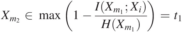 (15.1b)
where the mutual information I is symmetric.
I(Xm1; Xi) = H(Xm1) − H(Xm1| Xi)IXm1Xi=HXm1−HXm1Xi(15.1c)
3. Determine the third station (Xm3)Xm3) conditioning on Xm1and Xm2Xm1andXm2 by minimizing the transinformation (mutual information in a multivariate case) or maximize the coefficient of nontransformed information:
Xm3 ∈ min (H(Xm1, Xm2) − H(Xm1, Xm2| Xi)), i = 1, …, M, i ∉ (m1, m2)Xm3∈minHXm1Xm2−HXm1Xm2Xi,i=1,…,M,i∉m1m2(15.2a)
Comparing with Equation (15.1c), Equation (15.2a) is equivalent to
or
Xm3 ∈ min (I((Xm1, Xm2); Xm3)), i = 1, …, M, i ∉ (m1, m2)Xm3∈minIXm1Xm2Xm3,i=1,…,M,i∉m1m2(15.2b)
Xm3∈max1−HXm1Xm2−HXm1Xm2XiHXm1Xm2=t2,i=1,…,M,i∉m1m2 (15.2c)
4. Similarly, one can determine XmiXmi using Xmi ∈ min (H(Xm1, …, Xmi − 1)–H(Xm1, …, X_(mi − 1)| Xi))Xmi∈minHXm1…Xmi−1–HXm1…X_mi−1Xi
or
∈ min (I((Xm1, …, Xmi − 1); Xi)), i = 1, …, M, i ∉ (m1, …, mi − 1)∈minIXm1…Xmi−1Xi,i=1,…,M,i∉m1…mi−1(15.3a)
Xmi∈max1−HXm1…Xmi−1−HXm1…Xmi−1XmiHXm1…Xmi−1=ti−1 (15.3b)


The coefficient of nontransformed information should fulfill the following condition:
No more station is needed when ti ≤ ti + 1ti≤ti+1, i.e., the repetitive information exists at station Xmi + 1Xmi+1 such that only first Xm1, …, XmiXm1,…,Xmi stations are necessary for the network with initial M stations. In what follows, we will describe the procedure of rainfall network design using the procedures discussed in this section.
15.3.2 Estimation of Marginal Entropy
As stated in Section 15.3.1, the marginal entropy needs to be first estimated, and the station that yields the largest entropy will be chosen as the center station. As stated earlier, the empirical kernel density is applied to model the marginal rainfall variables in order to avoid the possible probability distribution misidentification. Furthermore, with the characteristic of rainfall records, the kernel density with the positive support is applied for analysis.
Following Beirlant et al. (2001), the marginal entropy is written as follows:
 (15.5)
where HmiHmi represents the marginal entropy of rain gauge mimi; n represents the length of rainfall record; and fmiker represents the kernel density function with positive supports.
15.3.3 Estimation of Mutual Information and Coefficient of Nontransferrable Information
In Chapter 8, we have discussed that the mutual information between two correlated random variables (X, Y) may be expressed through the copula entropy as follows:
and Equation (15.1b) may be rewritten through the copula entropy as follows:
 (15.7)
As stated in Yang and Burn (1994) and Alfonso et al. (2010), −HC(u, v)/H(Xm1)−HCuv/HXm1 represents the information inferred by first station m1m1 for another station Xi, i≠m1Xi,i≠m1 (on in other words, the information of m1m1 maintained in Xi, i≠m1Xi,i≠m1).
In a similar vine, the general equation (i.e., Equation (15.3a)) may be written as follows:
 (15.8a)
Applying the copula theory to Equation (15.8a), we have the following:
where Uj=FmjnXmj,j=1,…,i−1 is estimated from the kernel density with the positive support.
 (15.8c)
Equation (15.8a) may be written using the copula entropy as follows:
 (15.9)
and Equation (15.3b) may be rewritten as follows:
 (15.10)
It is seen from Equations (15.8)–(15.10) that the copula theory has a unique advantage of separating the marginal distribution from its joint distribution such that one may easily compute the joint and conditional entropies through the summation of marginal entropy and copula entropy.
15.4 Evaluation of Rainfall Network
To evaluate the rainfall network using the rainfall stations in Table 15.1 and Figure 15.1, the meta-elliptic (meta-Gaussian and meta-Student t) copulas are applied for illustrative purposes. It is worth mentioning that one may apply other copulas, including empirical copulas, to evaluate the network design.
15.4.1 Evaluation of the Rainfall Network with All Rainfall Stations
Applying Equation (15.5) for the marginal entropy estimation with the use of kernel density, Table 15.3 lists the computed marginal entropy for all 10 stations located in Louisiana. Table 15.3 shows that station Slidell (located in East Central Louisiana) yields the largest marginal entropy. As a result, Slidell is chosen as the center (the first) rain gauge station in the network.
Table 15.3. Estimated marginal entropy for the annual rainfall variable.
| Stations | Marginal H | Stations | Marginal H |
|---|---|---|---|
| Abbeville | 7.0920 | Lake Charles | 7.0935 |
| Baton Rouge | 7.0760 | Leland Bowman | 7.1398 |
| Crowley | 6.9883 | Livington | 7.1209 |
| De Ridder | 7.2280 | Rockfeller | 7.1328 |
| Jennings | 6.9674 | Slidell | 7.2361 |
Applying Equation (15.6), Tables 15.4 and 15.5 list the mutual information of Slidell with respect to the rest of the stations with the fitted meta-Gaussian and meta-Student t copulas, respectively. Using Slidell versus Abbeville as an illustrative example, the mutual information between Slidell and Abbeville may be estimated using bivariate meta-Gaussian copula (θ = 0.542θ=0.542) by taking the expectation for the copula density (i.e., bivariate Gaussian density) in the logarithm domain (HC = − 0.17HC=−0.17), which results in the mutual information I = − HC = 0.17I=−HC=0.17. Applying the meta-Gaussian and meta-Student t copulas, Tables 15.4 and 15.5 yield similar results with De Ridder (located in Southwest Louisiana) identified as the second station needed in the network.
Table 15.4. Mutual information as well as parameter estimated with respect to rain gauge Slidell (meta-Gaussian copula).
| Stations | Copula parameter | II | Stations | Copula parameter | I |
|---|---|---|---|---|---|
| Abbeville | 0.542 | 0.17 | Lake Charles | 0.510 | 0.15 |
| Baton Rouge | 0.544 | 0.18 | Leland Bowman | 0.429 | 0.10 |
| Crowley | 0.685 | 0.32 | Livington | 0.716 | 0.36 |
| De Ridder | 0.233 | 0.03 | Rockfeller | 0.652 | 0.28 |
| Jennings | 0.696 | 0.33 |
Table 15.5. Mutual information as well as the parameter estimated with respect to rain gauge Slidell (meta-Student t copula).
| Stations | Copula parameter | II | Stations | Copula parameter | I |
|---|---|---|---|---|---|
| Abbeville | [0.639, 4.67E06] | 0.186 | Lake Charles | [0.605, 1.47E07] | 0.160 |
| Baton Rouge | [0.673, 3.18] | 0.243 | Leland Bowman | [0.529, 4.67E06] | 0.109 |
| Crowley | [0.764, 4.67E06] | 0.334 | Livington | [0.800, 7.80] | 0.389 |
| De Ridder | [0.299, 25.90] | 0.030 | Rockfeller | [0.726, 9.09] | 0.295 |
| Jennings | [0.772, 1.14E07] | 0.349 |
With Slidell and De Ridder identified as the first two stations, the third station may be identified using Equation (15.9) by setting i = 3i=3 and minimizing I(X1, X2| X3) = HC(U1, U2) − HC(U1, U2, U3)IX1X2X3=HCU1U2−HCU1U2U3, which is estimated similarly as the bivariate case. Using the stations Slidell, De Ridder, and Abbeville as an illustrative example, we compute the copula entropy of Slidell (U1), De Ridder (U2), and Abbeville (U3) with the fitted bivariate and trivariate meta-Gaussian copula as follows:
Bivariate (Slidell and De Ridder):
θ = 0.2329, HC(U1, U2) = − 0.0279θ=0.2329,HCU1U2=−0.0279;
Trivariate (Slidell, De Ridder, and Abbeville):
θ=10.23290.54240.232910.59070.54240.59071,HCU1U2U3=−Elncu1u2u3=−0.3970;Conditional mutual information (Slidell, De Ridder|Abbeville):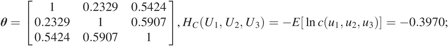
I(X1, X2| X3) = HC(U1, U2) − HC(U1, U2, U3) = − 0.0279 + 0.3970 = 0.3691.IX1X2X3=HCU1U2−HCU1U2U3=−0.0279+0.3970=0.3691.

Tables 15.6 and 15.7 list all the computed conditional mutual information using the fitted meta-Gaussian and meta-Student t copulas. As seen in Tables 15.6 and 15.7, the meta-Gaussian and meta-Student t copulas again are in agreement that Baton Rouge is the third station needed.
Table 15.6. Mutual information computed with respect to rain gauges Slidell (X1)X1) and De Ridder (X2)X2) (meta-Gaussian copula).
| X1, X2 ∣ X3X1,X2∣X3 | −HC(X1, X2) = I(X1, X2) = 0.0279−HCX1X2=IX1X2=0.0279 | ||
|---|---|---|---|
| I(X1, X2| Abbeville)IX1X2Abbeville | 0.369 | I(X1, X2| Lake Charles)IX1X2Lake Charles | 0.388 |
| I(X1, X2| Baton Rouge)IX1X2Baton Rouge | 0.177 | I(X1, X2| Leland Bowman)IX1X2Leland Bowman | 0.286 |
| I(X1, X2| Crowley)IX1X2Crowley | 0.414 | I(X1, X2| Livgington)IX1X2Livgington | 0.360 |
| I(X1, X2| Jennings)IX1X2Jennings | 0.508 | I(X1, X2| Rockfeller)IX1X2Rockfeller | 0.364 |
Table 15.7. Mutual information computed with respect to rain gauges Slidell (X1)X1) and De Ridder (X2)X2 (meta-Student t copula).
| X1, X2 ∣ X3X1,X2∣X3 | −HC(X1, X2) = I(X1, X2) = 0.0279−HCX1X2=IX1X2=0.0279 | ||
|---|---|---|---|
| I(X1, X2| Abbeville)IX1X2Abbeville | 0.369 | I(X1, X2| Lake Charles)IX1X2Lake Charles | 0.388 |
| I(X1, X2| Baton Rouge)IX1X2Baton Rouge | 0.177 | I(X1, X2| Leland Bowman)IX1X2Leland Bowman | 0.286 |
| I(X1, X2| Crowley)IX1X2Crowley | 0.414 | I(X1, X2| Livgington)IX1X2Livgington | 0.360 |
| I(X1, X2| Jennings)IX1X2Jennings | 0.508 | I(X1, X2| Rockfeller)IX1X2Rockfeller | 0.364 |
Proceeding with the same procedure, we will add more stations to the network until the criterion described in Equation (15.4) is no longer valid. The final results are listed in Table 15.8 using the fitted meta-Gaussian copula as an example. The same stations are obtained with the use of the Student t copula. Figure 15.3 plots the identified rain gauges on the map. As shown in Figure 15.3, all three rain gauges located in East Central Louisiana are needed for rainfall network design, while only two of seven rain gauges are needed for those located in Southwest Louisiana. This information may indicate more uncertainty within East Central Louisiana than that within Southwest Louisiana.
Table 15.8. Final results for the rainfall network design (meta-Gaussian copula).
| Stations already identified | Station added | H(X1, .., Xi)HX1..Xi | H(X1, …, Xi| Xi + 1)HX1…XiXi+1 | I((X1, …, Xi); Xi + 1)IX1…XiXi+1 | tt |
|---|---|---|---|---|---|
| — | Slidell | 7.236 | — | — | 1 |
| Slidell | De Ridder | 7.236 | 7.208 | 0.0279 | 0.996 |
| Slidell, De Ridder | Baton Rouge | 14.436 | 14.259 | 0.177 | 0.987 |
| Slidell, De Ridder Baton Rouge | Leland Bowman | 21.336 | 20.969 | 0.367 | 0.983 |
| Slidell, De Ridder Baton Rouge, Leland Bowman | Livington | 28.108 | 27.519 | 0.589 | 0.979 |

15.4.2 Evaluation of Rain Gauges Located in Southwest Louisiana Only
From Figure 15.1, there are seven stations located in the Southwest region. Applying the same procedure as that for all the rain gauges, we can identify the rain gauges needed for the Southwest region only. Table 15.9 lists the final four identified rain gauges with the use of the meta-Gaussian copula as an example. Figure 15.4 maps the stations identified for the Southwest region. Comparing to the final result of the Southwest region with that for combined Southwest and East Central regions, station De Ridder is identified in both cases. In addition, there is only about 19-mile distance between Leland Bowman (selected for Southwest and East Central only) and Abbeville (Southwest only).
Table 15.9. Final results for rainfall network design (Southwest region) (meta-Gaussian copula).
| Stations already identified | Station added | H(X1, .., Xi)HX1..Xi | H(X1, …, Xi| Xi + 1)HX1…XiXi+1 | I((X1, …, Xi); Xi + 1)IX1…XiXi+1 | tt |
|---|---|---|---|---|---|
| — | De Ridder | 7.228 | — | — | 1 |
| De Ridder | Rockfeller | 7.228 | 7.117 | 0.112 | 0.985 |
| De Ridder, Rockfeller | Crowley | 14.249 | 13.881 | 0.368 | 0.974 |
| De Ridder, Rockfeller | Abbeville | 20.87 | 20.275 | 0.595 | 0.972 |
| Crowley |

Figure 15.4 Final identification of rain gauges needed for Southwest Louisiana (retrieved from http://maps.google.com).
15.5 Summary
In this case study, rain gauges located in the East Central and Southwest regions of Louisiana are applied for the rainfall network design. Considering the East Central and Southwest regions together, the needed rain gauges reduce from 10 to 5. All three rain gauges in the East Central region are needed, while only De Ridder and Leland Bowman (about 19 miles southwest of Abbeville) are needed for the Southwest region.
Considering Southwest Louisiana only, four out of seven stations are needed. Of the four stations needed, station De Ridder is the common station identified for both cases. Besides the De Ridder station, the fourth added station (Abbeville) is geographically close to Leland Bowman station.
The spatial distribution of rain gauges, for the East Central and Southwest regions, and the Southwest region only, well covers the region studied respectively. Investigation of the network results in the reduction of the number of rain gauges.
Application of the empirical marginal distributions (kernel density) for the marginal rainfall may avoid the misidentification of the marginal distributions. Application of the copula theory eases the complexity of estimating the joint and conditional entropies; in higher dimensions, the estimation may be made by separately assessing the marginal entropy and the copula entropy.
The network design with the copula theory may be applied not only in the rainfall network, it may also be easily applied to other network design problems (streamflow gauges, sewer monitoring program, etc.). In addition, it may be applied to add an additional point if the current monitor program may not properly represent the system.