Abstract
In this chapter, we will introduce the last application of the book, i.e., interbasin transfer. In this process, there are two main components: donor and receiver basins. The purpose of interbasin transfer to redistribute water from a water-rich region to the region with water shortage. The interbasin transfer may help reducing the impact of dry conditions in the region with water shortage.
17.1 Case-Study Site and Dataset
In this chapter, we will provide a synthetic analysis for interbasin transfer using the river systems in Texas, the United States, as an example. Based on the description of Texas, the climate in Texas varies from arid in the west to humid in the east (as shown in Figure 17.1). The major river systems as well as major cities are shown in Figure 17.1. Among all the major river systems, the Brazos, Sabine, and Trinity Rivers carry the largest annual runoff of 6,074,000; 5,864,000; and 5,127,000 acre feet, respectively. Climatewise, the eastern coastal region is in the tropic humid climate region with abundant precipitation throughout the year. However, the central and western parts of Texas are within the arid/semi-arid climate region and may not receive enough precipitation. Thus, it is viable to transport the abundant water from the eastern part of Texas to central and western parts of Texas under the conditions of no or minimum negative impact on the highly developed eastern coastal area of Texas. In this case study, we will choose Lake Houston (USGS 08072000) as a donor reservoir, and E. V. Spence Reservoir (USGS 08123950) as a receiver reservoir to evaluate the possibility of interbasin transfer.
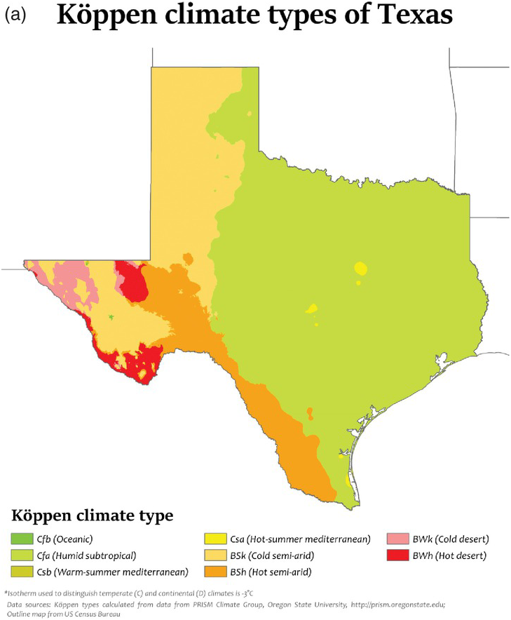
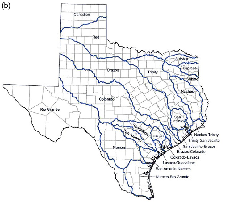
Figure 17.1 (a) Köppen climate types of Texas (retrieved from https://commons.wikimedia.org/wiki/File:Texas_K%C3%B6ppen.svg).
(b) Major rivers and cities in Texas (retrieved from www.twdb.texas.gov/surfacewater/rivers/index.asp, courtesy of Texas Water Development Board).
Lake Houston was constructed in 1953 and is currently serving as the primary source of water supply for the city of Houston. The E. V. Spence Reservoir is located west of Robert Lee, Texas. In the normal years, the E. V. Spence Reservoir may be sufficient to provide the water supply for Robert Lee and surrounding communities in Coke County. However, during the recent drought, the reservoir storage decreased to less than 0.76% of its capacity. As of June 2016, the lake was back up to 10.4% of its capacity (Wikipedia.org). To illustrate the process, monthly storage is applied. The full capacity storage of Lake Houston is 134,313 acre feet. The full capacity storage of the E. V. Spence Reservoir is 135,704 acre feet. Based on the availability of the dataset (USGS), the data from water year of 2000 to 2016 are applied for analysis. In addition, there is one data value missing for Lake Houston (May 2015) and one for E. V. Spence Reservoir (May 2004). The missing value at Lake Houston and E. V. Spence Reservoir is filled based on the recent drought. The missing value at Lake Houston is filled with the average flow of May, while the missing value at E.V. Spence Reservoir is filled with the average flow of May before water year 2010 (i.e., before the 2010–2013 drought in the southern United States and Mexico). The entire dataset is listed in Table 17.1.
Table 17.1. Storage at Lake Houston and E. V. Spence Reservoir (acre feet).
| Year | Month | USGS08072000 | USGS08123950 | Year | Month | USGS0807200 | USGS08123950 |
|---|---|---|---|---|---|---|---|
| 2000 | 10 | 100,800 | 83,700 | 2008 | 10 | 141,900 | 59,510 |
| 2000 | 11 | 136,800 | 88,260 | 2008 | 11 | 143,700 | 56,880 |
| 2000 | 12 | 144,200 | 86,270 | 2008 | 12 | 142,600 | 54,680 |
| 2001 | 1 | 147,200 | 84,840 | 2009 | 1 | 140,600 | 52,590 |
| 2001 | 2 | 145,400 | 83,870 | 2009 | 2 | 137,700 | 51,010 |
| 2001 | 3 | 144,600 | 82,740 | 2009 | 3 | 141,600 | 49,320 |
| 2001 | 4 | 144,100 | 80,930 | 2009 | 4 | 145,100 | 46,400 |
| 2001 | 5 | 141,600 | 78,060 | 2009 | 5 | 143,100 | 43,710 |
| 2001 | 6 | 147,400 | 74,020 | 2009 | 6 | 134,300 | 40,920 |
| 2001 | 7 | 143,500 | 69,470 | 2009 | 7 | 134,900 | 37,290 |
| 2001 | 8 | 140,200 | 64,540 | 2009 | 8 | 137,200 | 34,180 |
| 2001 | 9 | 143,500 | 61,800 | 2009 | 9 | 138,600 | 31,080 |
| 2001 | 10 | 140,600 | 58,570 | 2009 | 10 | 144,700 | 28,530 |
| 2001 | 11 | 134,000 | 58,300 | 2009 | 11 | 144,400 | 26,170 |
| 2001 | 12 | 148,300 | 61,510 | 2009 | 12 | 145,700 | 24,840 |
| 2002 | 1 | 145,000 | 59,730 | 2010 | 1 | 143,300 | 23,950 |
| 2002 | 2 | 144,300 | 57,840 | 2010 | 2 | 143,700 | 24,410 |
| 2002 | 3 | 141,800 | 55,190 | 2010 | 3 | 142,600 | 23,900 |
| 2002 | 4 | 143,000 | 53,860 | 2010 | 4 | 140,300 | 22,990 |
| 2002 | 5 | 136,900 | 52,880 | 2010 | 5 | 141,600 | 25,400 |
| 2002 | 6 | 137,300 | 55,000 | 2010 | 6 | 142,700 | 25,100 |
| 2002 | 7 | 142,900 | 54,760 | 2010 | 7 | 143,500 | 24,530 |
| 2002 | 8 | 140,900 | 51,230 | 2010 | 8 | 137,100 | 22,680 |
| 2002 | 9 | 141,200 | 47,390 | 2010 | 9 | 140,600 | 19,950 |
| 2002 | 10 | 146,500 | 45,600 | 2010 | 10 | 132,300 | 20,810 |
| 2002 | 11 | 150,300 | 44,740 | 2010 | 11 | 134,800 | 18,550 |
| 2002 | 12 | 147,500 | 42,940 | 2010 | 12 | 133,100 | 16,360 |
| 2003 | 1 | 145,500 | 41,410 | 2011 | 1 | 142,100 | 14,600 |
| 2003 | 2 | 148,900 | 40,000 | 2011 | 2 | 138,300 | 13,650 |
| 2003 | 3 | 144,900 | 38,420 | 2011 | 3 | 136,300 | 12,060 |
| 2003 | 4 | 143,000 | 35,540 | 2011 | 4 | 130,300 | 10,130 |
| 2003 | 5 | 139,900 | 32,770 | 2011 | 5 | 118,600 | 8,026 |
| 2003 | 6 | 141,500 | 51,950 | 2011 | 6 | 106,600 | 6,104 |
| 2003 | 7 | 144,000 | 57,600 | 2011 | 7 | 99,040 | 4,027 |
| 2003 | 8 | 140,900 | 53,110 | 2011 | 8 | 87,870 | 2,847 |
| 2003 | 9 | 143,900 | 53,040 | 2011 | 9 | 84,700 | 2,500 |
| 2003 | 10 | 144,700 | 51,590 | 2011 | 10 | 96,990 | 2,362 |
| 2003 | 11 | 144,600 | 49,320 | 2011 | 11 | 114,400 | 2,231 |
| 2003 | 12 | 142,000 | 46,790 | 2011 | 12 | 136,500 | 2,194 |
| 2004 | 1 | 146,500 | 44,630 | 2012 | 1 | 141,700 | 2,249 |
| 2004 | 2 | 145,700 | 42,870 | 2012 | 2 | 144,800 | 2,323 |
| 2004 | 3 | 141,000 | 46,050 | 2012 | 3 | 143,800 | 2,320 |
| 2004 | 4 | 141,200 | 49,040 | 2012 | 4 | 139,000 | 2,215 |
| 2004 | 5 | 145,300 | 63,819 | 2012 | 5 | 134,900 | 2,100 |
| 2004 | 6 | 143,900 | 44,640 | 2012 | 6 | 137,300 | 1,839 |
| 2004 | 7 | 140,200 | 42,840 | 2012 | 7 | 143,700 | 1,463 |
| 2004 | 8 | 138,500 | 43,160 | 2012 | 8 | 139,100 | 1,164 |
| 2004 | 9 | 138,100 | 43,590 | 2012 | 9 | 131,800 | 1,111 |
| 2004 | 10 | 123,300 | 39,490 | 2012 | 10 | 135,700 | 28,440 |
| 2004 | 11 | 146,400 | 53,810 | 2012 | 11 | 131,900 | 28,840 |
| 2004 | 12 | 143,700 | 79,410 | 2012 | 12 | 128,600 | 28,480 |
| 2005 | 1 | 144,500 | 78,630 | 2013 | 1 | 138,300 | 27,800 |
| 2005 | 2 | 150,000 | 78,460 | 2013 | 2 | 139,800 | 27,210 |
| 2005 | 3 | 143,500 | 78,490 | 2013 | 3 | 135,400 | 26,000 |
| 2005 | 4 | 141,200 | 76,190 | 2013 | 4 | 139,100 | 24,790 |
| 2005 | 5 | 140,300 | 73,600 | 2013 | 5 | 138,900 | 23,370 |
| 2005 | 6 | 139,600 | 72,450 | 2013 | 6 | 139,800 | 26,680 |
| 2005 | 7 | 141,600 | 68,290 | 2013 | 7 | 134,000 | 28,510 |
| 2005 | 8 | 141,900 | 85,160 | 2013 | 8 | 132,800 | 27,570 |
| 2005 | 9 | 133,800 | 101,900 | 2013 | 9 | 132,300 | 25,770 |
| 2005 | 10 | 138,300 | 99,360 | 2013 | 10 | 141,700 | 24,170 |
| 2005 | 11 | 138,700 | 97,300 | 2013 | 11 | 140,900 | 22,800 |
| 2005 | 12 | 141,700 | 94,870 | 2013 | 12 | 140,200 | 20,990 |
| 2006 | 1 | 140,600 | 92,960 | 2014 | 1 | 139,300 | 19,030 |
| 2006 | 2 | 142,800 | 91,210 | 2014 | 2 | 139,900 | 17,400 |
| 2006 | 3 | 140,700 | 89,790 | 2014 | 3 | 143,300 | 15,550 |
| 2006 | 4 | 140,100 | 88,650 | 2014 | 4 | 138,100 | 13,410 |
| 2006 | 5 | 142,300 | 87,120 | 2014 | 5 | 140,600 | 11,330 |
| 2006 | 6 | 143,200 | 82,880 | 2014 | 6 | 143,500 | 11,790 |
| 2006 | 7 | 142,900 | 77,900 | 2014 | 7 | 141,400 | 10,450 |
| 2006 | 8 | 140,900 | 72,880 | 2014 | 8 | 136,500 | 8,627 |
| 2006 | 9 | 138,700 | 76,020 | 2014 | 9 | 138,300 | 8,025 |
| 2006 | 10 | 146,700 | 73,890 | 2014 | 10 | 140,100 | 14,670 |
| 2006 | 11 | 136,700 | 71,120 | 2014 | 11 | 137,400 | 13,040 |
| 2006 | 12 | 135,400 | 69,300 | 2014 | 12 | 140,700 | 11,760 |
| 2007 | 1 | 140,300 | 68,460 | 2015 | 1 | 143,300 | 10,730 |
| 2007 | 2 | 134,300 | 67,650 | 2015 | 2 | 139,400 | 10,460 |
| 2007 | 3 | 140,400 | 67,200 | 2015 | 3 | 143,800 | 96,50 |
| 2007 | 4 | 141,900 | 70,340 | 2015 | 4 | 143,200 | 11,410 |
| 2007 | 5 | 144,100 | 74,250 | 2015 | 5 | 140,330 | 18,260 |
| 2007 | 6 | 143,300 | 74,490 | 2015 | 6 | 145,500 | 28,370 |
| 2007 | 7 | 138,600 | 72,600 | 2015 | 7 | 141,100 | 38,570 |
| 2007 | 8 | 136,500 | 77,170 | 2015 | 8 | 137,800 | 39,670 |
| 2007 | 9 | 134,300 | 84,430 | 2015 | 9 | 140,100 | 36,760 |
| 2007 | 10 | 134,200 | 80,920 | 2015 | 10 | 134,300 | 37,830 |
| 2007 | 11 | 138,100 | 77,460 | 2015 | 11 | 144,600 | 46,240 |
| 2007 | 12 | 140,400 | 75,980 | 2015 | 12 | 145,400 | 50,110 |
| 2008 | 1 | 140,200 | 74,570 | 2016 | 1 | 144,300 | 50,840 |
| 2008 | 2 | 143,700 | 72,700 | 2016 | 2 | 141,800 | 49,390 |
| 2008 | 3 | 144,100 | 71,540 | 2016 | 3 | 147,400 | 48,020 |
| 2008 | 4 | 141,500 | 70,370 | 2016 | 4 | 151,100 | 48,130 |
| 2008 | 5 | 142,400 | 68,160 | 2016 | 5 | 154,400 | 51,810 |
| 2008 | 6 | 138,200 | 66,990 | 2016 | 6 | 150,100 | 53,790 |
| 2008 | 7 | 135,400 | 65,340 | 2016 | 7 | 142,100 | 53,430 |
| 2008 | 8 | 141,300 | 63,400 | 2016 | 8 | 144,200 | 50,120 |
| 2008 | 9 | 144,000 | 62,440 | 2016 | 9 | 143,100 | 49,630 |
With the collected reservoir storage dataset listed in Table 17.1, the procedure to assess the interbasin transfer is outlined as follows:
i. Investigate the univariate time series.
ii. Apply the time series-copula approach to study the bivariate analysis.
iii. Set the rule for interbasin transfer and assess the interbasin transfer probability using the time series-copula developed in step ii.
17.2 Investigation of Univariate Storage Time Series
Given that monthly reservoir storage may not be considered a random variable, the autocorrelation and partial autocorrelation are plotted in Figure 17.2 first to evaluate the stochastic behavior of the monthly storage at USGS08072000 (Lake Houston) and at USGS08123950 (E. V. Spence Reservoir). In Figure 17.2, we see the following:
1. There is no obvious seasonality at both locations.
2. The storage at USGS08072000 (Lake Houston) may be considered a stationary signal.
3. The storage at USGS08123950 (E. V. Spence Reservoir) is clearly nonstationary.

Figure 17.2 Sample autocorrelation and partial autocorrelation plots for the stations at Lake Houston and E. V. Spence Reservoir.
Table 17.2 lists the sample statistics of the storage series. The sample statistics show that the storage series is clearly skewed with a heavy tail. In addition to the sample statistics listed in Table 17.2, the histogram plotted in Figure 17.3 also suggests that the storage series at both locations do not follow the Gaussian process.
Table 17.2. Sample statistics of observed the storage series at USGS08072000, US08123950, as well as USGS08123950 after the first-order difference.
| Station | Mean | Standard deviation | Skewness | Kurtosis |
|---|---|---|---|---|
| USGS08072000 | 139311.98 | 9335.10 | –3.52 | 17.98 |
| USGS08123950 | 45319.61 | 26711.91 | 0.04 | 1.95 |

Figure 17.3 Histogram of observed storage series.
As a result, we are applying the meta-Gaussian transformation to the storage series before we proceed. To avoid the future interpolation of the order series discussed in Ayra and Zhang (2014), the kernel density approach is adopted here to assess the univariate distribution rather than the empirical distribution with plotting position. The univariate storage time series is then transformed as follows:
1. Apply the kernel density with positive support to estimate the empirical CDF of Si as Fn(Si)FnSi.
2. Apply the meta-Gaussian transformation to obtain the transformed storage variable SiT
 as
as
SiT=Φ−1FnSi01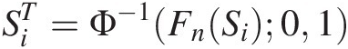 (17.1)


With the application of meta-Gaussian transformation, Figure 17.4 plots the histogram of storage time series after transformation. Figure 17.5 plots the sample autocorrelation and partial autocorrelation of the transformed storage series at USGS08072000, USGS08123950, and USGS08123950 after the first-order differencing. Figure 17.4 shows that the transformed series is now closer to the Gaussian process. Figure 17.5 shows that the overall structure of the time series is not changed after transformation. Thus, we can safely study the transformed series as a representation for the observed storage series directly. As shown in Figure 17.3 and Figure 17.5, the AR(1) model may be applied to both the transformed storage at USGS08072000 and the first-order differenced transformed storage at USGS08123950 with parameters estimated as listed in Table 17.3. The diagnostics are given in Table 17.4 for the assessment of linear independence (Ljung-Box Q-test), second-order independence (ARCH test), and white Gaussian noise test for the model residuals. The results in Table 17.4 show that the normality test for USGS08123950 fails even after the application of meta-Gaussian transformation; however, the parameters listed in Table 17.3 are still valid estimates for USGS08123950 if the model residual may be fitted using the stable distribution (DuMouchel, 1973). Applying the stable distribution, the parameters estimated for the model residual at USGS08123950 are as follows:
After performing the KS goodness-of-fit study, we have D = 0.042, P = 0.8799D=0.042,P=0.8799. To this end, we have successfully constructed the univariate time series model for the storage time series at USGS08072000 and USGS08123950 as follows:
1. The AR(1) model may properly model the storage series at USGS08072000 after the meta-Gaussian transformation.
2. ARIMA(1,1,0) with stable distributed residues may properly model the storage series at USGS08123950 after the meta-Gaussian transformation.

Figure 17.4 Histogram of storage series after meta-Gaussian transformation.

Figure 17.5 Sample autocorrelation and partial autocorrelation of the transformed series.
Table 17.3. Parameter estimated for univariate storage time series.
| Station | Model | cc | ϕϕ | Variance (σe2) |
|---|---|---|---|---|
| USGS08072000 | AR(1) | –0.0018 | 0.637 | 0.55 |
| USGS08123950 | ARIMA(1,1,0) | –0.004 | 0.149 | 0.04 |
Table 17.4. Diagnostic test for model residuals.
| Diagnostic | LBQ (H, P) | ARCH (H, P) | N0σe2 |
|---|---|---|---|
| USGS08072000 | [0, 0.87] | [0, 0.33] | [0, 0.80] |
| USGS08123950 | [0, 0.96] | [0, 0.84] | [1, 0] |
17.3 Investigation of Storage at USGS08072000 and USGS08123950 with Bivariate Analysis
With the univariate time series constructed, we will now be able to study their joint dependence structure and assess the possible water transfer from USGS08072000 (Lake Houston) to USGS08123950 (E. V. Spence Reservoir) by applying copulas to the fitted model residuals. The Kendall correlation coefficient computed with the use of the fitted model residuals at both locations is computed as τn = 0.087τn=0.087. From the computed Kendall correlation, it is seen that USGS08072000 and USGS08123950 are close to being independent. This may be understood by the different climate regions of USGS08072000 (Lake Houston: humid) and USGS08123950 (E. V. Spence Reservoir, semi-arid).
Applying the Frank, Clayton, and Gaussian copula, Figure 17.6 plots the comparison of simulated random variables from the copula candidates to the fitted model residuals. As seen from Figure 17.6, there are no visually significant differences among three copula functions. Table 17.5 lists the estimated parameters as well as the GoF results with the Rosenblatt transform (Genest et al., 2007). Based on the GoF results, all three copula candidates pass the test, with the Clayton copula yielding the smallest test statistics. Thus, the Clayton copula is chosen for further assessment.

Figure 17.6 Comparison of marginals from the fitted model residuals to the random variables simulated from the fitted copula candidates.
Table 17.5. Parameter and GoF results for the fitted copula functions.
| Copula | Frank | Clayton | Gaussian |
|---|---|---|---|
| Parameter (θθ) | 1.076 | 0.274 | 0.156 |
Gof(SnB,Pvalue ) ) | (0.085, 0.241) | (0.049, 0.299) | (0.072, 0.253) |
17.4 Assessment of Interbasin Transfer
The interbasin transfer is evaluated using the following rules:
1. No interbasin transfer will be allowed if the storage at donor (USGS08072000: Lake Houston) is less than 70% of its capacity.
2. Interbasin transfer will be allowed if the storage at donor is greater than 70% of its capacity and the storage at the receiver (USGS08123950) is less than 30%.
3. Interbasin transfer is not necessary if the storage at receiver is higher than 60% of its capacity.
With the preceding rules, we know the univariate analysis may be applied to evaluate rules 1 and 3, and the bivariate study will be needed for rule 2. Now to evaluate rule 2, we may compute the joint probability of PSrt≤0.4SrFull∩Sdt≥0.7SdFull and the conditional probability of PSdt≥0.7SdFullSrt≤0.4SrFull
 as follows:
 (17.2)
 (17.3)
In Equations (17.2) and (17.3), the marginals are evaluated from the univariate time series model through the fitted model residuals as follows:


Additionally, from the raw data, we see 190 out of 192 months with the storage higher than 70% of the capacity (except September and October of 2011) at USGS08072000 (Lake Houston). However, 121 out of 192 months were found with storage less than 40% of the capacity at USGS 08123950 (E. V. Spence Reservoir). To this end, we conclude that it is viable to transfer the water from Lake Houston to E. V. Spence Reservoir without imposing negative impacts on the communities served by Lake Houston.
Let R = 1 (no transfer is available) if the storage at USGS0807000 is less than 70% for rule 1; and R = 0 (no transfer is necessary) if the storage at USGS08123950 is greater than 60% for rule 3. In the case of rule 2, the joint probability and conditional probability are computed using Equations (17.2) and (17.3). Figure 17.7 plots the probability of rule 2 in conjunction of rules 1 and 3. Figure 17.7 indicates the following:
1. The receiver reservoir (USGS08123950) may not receive any water from the donor (USGS08072000) for September and October of 2011 regardless of the situation of the receiver reservoir, due to insufficient water storage in the donor reservoir.
2. The receiver reservoir has enough water, and no interbasin transfer is necessary for the periods of October 2000–July 2002, July 2003, April 2005, and December 2004–December 2008.
3. The receiver reservoir is in need of water from the donor Lake Houston. It is seen for most cases that the receiver may receive water from Lake Houston except for September and October of 2011. This coincides with the southern and Mexico drought of 2010–2013, and Lake Houston itself was experiencing the decrease of the storage due to drought.

Figure 17.7 Probability of rule 2 and in conjunction with rules 1 and 3.
17.5 Forecast of Interbasin Transfer
In this section, we will provide a simple example to illustrate the procedure of interbasin transfer forecast.
1. One-month ahead storage forecast with the use of the fitted univariate time series model for the time series with meta-Gaussian transformation (i.e., SDT/SRT
 ):
):
USGS08072000:
The forecast equation may be written as follows:
SDTt+1=cD+ϕDSDTt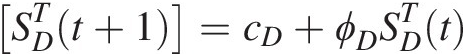 (17.4)
Substituting c=−0.0018,ϕ=0.637SDT192=0.4835
 into Equation (17.4), we have the following:
Oct.2016:SDTt+1=SDT193=−0.0018+0.6370.4835=0.3062With the results obtained from the meta-Gaussian transformation, we may reestimate the storage of USGS08072000 through its inverse:
With the probability computed in the preceding, we may finally estimate the storage for October 2016 through the kernel density function as follows:
P = Φ(0.3062, 0, 1) = 0.6203P=Φ0.306201=0.6203
USGS08123950:
SD(Oct. 2016) = 142410 acre. ft = 1.06 full capacity of Lake Houston (134313 acre. ft)SDOct.2016=142410acre.ft=1.06full capacity of Lake Houston134313acre.ft
Similar to that for USGS8072000, the forecast equation for USGS081239500 may be written as follows:
SRTt+1=cR+1+ϕRSRTt−ϕRSRTt−1Substituting cR=−0.004,ϕR=0.149,SRT192=0.1646;SRT191=0.1791 (17.5)
 into Equation (17.5), we have the following:
SRTOct.2016=0.1583;P=Φ0.1583=0.5629;Finally, we have
SR(Oct.2016) = 50877 acre. ft = 0.37 full capacity of E. V. Spence Reservoir (135704 acre. ft).SROct.2016=50877acre.ft=0.37full capacity ofE.V.Spence Reservoir135704acre.ft.
2. Probability of interbasin transfer for the coming month.


Previously we have estimated the storage for October 2016 as 142,410 acre feet and 5,0877 acre feet for Lake Houston (USGS08072000) and E. V. Spence Reservoir (USGS08123950), respectively. As compared to the full capacity of Lake Houston and E. V. Spence Reservoir, the storage condition falls into rule 2, that is, water is needed from Lake Houston to replenish E. V. Spence Reservoir. Based on rule 2, we can further compute the corresponding joint and conditional probability. It is known that when we proceed for the forecast, we assume et = 0et=0 for median forecast.
As discussed earlier, the USGS08072000 may be fitted by the classic AR(1) model with Gaussian white noise and we have PD(et) = N(0, 0, 0.545) = 0.5PDet=N000.545=0.5. For the stable distribution-driven ARIMA(1,1,0) model for USGS08123950, we can compute the probability numerically as PR(et) = 0.7349PRet=0.7349.
Finally we have the joint probability and conditional probability as R1 = 0.348 and R2 = 0.473. The probability obtained for rule 2 tells us the following:
i. The probability of the receiver having less storage (i.e., the storage being less than 40%) and the storage at the donor being higher than the estimated storage above the 70% cutoff limit is about 34.8% (i.e., R1).
ii. The probability of donor with storage higher than 70% given the receiver basin with less than 30% (full storage) is about 47.3% (i.e., R2).
iii. The probability computed suggests the preparation for basin transfer.
17.6 Summary
In this chapter, we introduced the applications of copula to interbasin transfer study. Applying USGS08072000 (Lake Houston) and USGS08123950 (E. V. Spence Reservoir) as an example, the near real-time interbasin transfer is explained. Lake Houston is located in southeastern Texas within the humid climate region, while E. V. Spence Reservoir is located in central western Texas within the semi-arid region. In this case study, the monthly storage is applied for analysis. The seasonality is not found within the storage series. The analysis shows the following:
With the highly skewed and heavy tailed structure of the time series, the meta-Gaussian transformation is first applied with the empirical frequency assessed by the kernel density function with positive support.
The storage at USGS08072000 is stationary, while the storage at USGS08123950 is nonstationary. This may be understood, as for the humid region in Texas, the overall weather pattern throughout the year is more consistent than in central western Texas in the semi-arid region.
With the meta-Gaussian transformation, the AR(1) model with white Gaussian noise may be applied to model the storage series at USGS08072000, and ARIMA(1,1,0) with stable distributed noise may be applied to model the storage series at USGS08123950.
With the storage series being time series rather than the random variable, the copula is applied to the model residuals, which are random.
Application of copula to the model residuals shows that the fitted model residuals at two locations is about 0.087, which is close to being independent. This is understandable due to the geographical distance as well as different climate regions.
With the time series copula approach, it is possible to forecast the probability of interbasin transfer of the following month with the use of one-month ahead forecast.