Abstract
Bivariate or multivariate frequency analysis entails univariate distributions that are determined by empirical fitting to data. The fitting, in turn, requires the determination of distribution parameters and the assessment of the goodness of fit. In practical applications, such as hydrologic design, risk analysis is also needed. The objective of this chapter, therefore, is to briefly discuss these basic elements, which are needed for frequency analysis and will be needed in subsequent chapters.
2.1 Univariate Probability Distributions
Among the univariate distributions, we will briefly discuss the most commonly applied continuous univariate distributions, especially in univariate hydrological frequency analyses (Kite, 1977; Singh, 1998; Rao and Hamed, 2000; Singh and Zhang, 2016). In what follows, we will use X as an independent identically distributed (IID) random variable with probability density function (PDF) f(x)fx and cumulative distribution function (CDF) F(x)Fx.
2.1.1 Normal Distribution
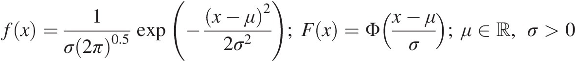
Normal distribution: The PDF and CDF of the normal distribution can be given as follows:
 (2.1)
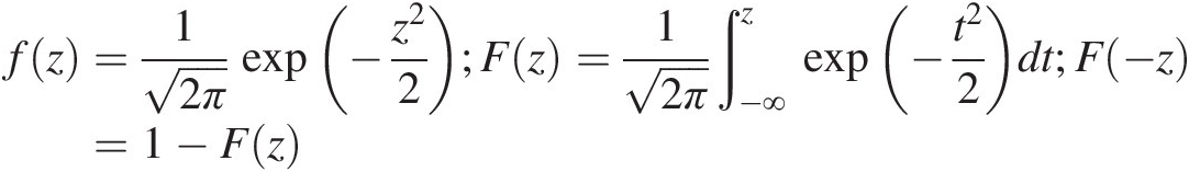
(2.1)In Equation (2.1), ΦΦ represents the standard normal distribution, and μ, σμ,σ are the location and scale parameters having the connotation of mean and standard deviation of the random variable, respectively. Defining the standard normal variable z = (x − μ)/σz=x−μ/σ, Equation (2.1) can be written as
 (2.1a)
Abramowitz and Stegun (1965) have numerically approximated F(z) with an error less than 7.5 × 10−57.5×10−5 as
where a1 − 0.319381530, a2 = − 0.356563782, a3 = 1.781477937, a4 = − 1.821255978, a5 = 1.330274429a1=−0.319381530,a2=−0.356563782,a3=1.781477937,a4=−1.821255978,a5=1.330274429, and ϵ(z)ϵz is the error of approximation.
In hydrological frequency analysis, the normal distribution has been commonly applied in two scenarios:
1. Normal distribution with mean of zero is the classic assumption for time series analysis and regression analysis. As a simple example, let Y be the response or prediction variable and X be the predictor variable. Then, a simple linear regression can be expressed as
EYX=Ŷ=a+bx;e=Y−Ŷande~N0σe2where e is the residual or error and e~N0σe2 (2.2)
(2.2) denotes that e is distributed normally with mean 0 and variance σe2.
 E[Y| X]EYX denotes the conditional expectation of Y given X. Ŷ
 denotes the predicted response through simple linear regression with intercept of a and slope of b.
For example, a stationary time series {Xt, t = 1, 2, …}Xtt=12… modeled by an Autoregressive and Moving Average (ARMA) model with (p, q) (Box et al., 2007) as follows:
xt=c+ϕ1xt−1+…+ϕpxt−p+et+θ1et−1+…+θqet−q;et~N0σet2 (2.3)
(2.3)
In Equation (2.3), c is the long-term average of the time series, and ϕ1, …, ϕp; θ1, …, θqϕ1,…,ϕp;θ1,…,θq are, respectively, the coefficients for autoregressive and moving average terms. More specifically, in Equations (2.2) and (2.3), the residual e, following normal distribution with mean of 0 is commonly called white Gaussian noise.
2. After certain monotone transformation (e.g., Box–Cox or probability integral transformation), the normal distribution (Equation (2.1)) may be applied to model the nonnormally distributed hydrologic variables (e.g., Hazen, 1914; Markovic, 1965).


2.1.2 Log-Normal Distribution
Let Y = ln (x).Y=lnx. If X follows the log-normal distribution, then its logarithm follows the normal distribution, whose PDF can be written as follows:
 (2.4)
(2.4)The CDF of the log-normal distribution can be computed again through the standard normal distribution as follows:
 (2.5)
(2.5)The logarithm of the random variable X is a special case of the Box–Cox transformation (Box and Cox, 1964) with λ = 0λ=0:
 (2.5a)
The log-normal distribution has been widely used in hydrological frequency analysis (e.g., Chow, 1954).
2.1.3 Student t Distribution
Similar to the normal distribution, the Student t distribution is also bell-shaped (Hogg and Craig, 1978). However, it possesses the heavy tail, i.e., excess kurtosis is greater than 0. The PDF of the standard Student t distribution is given as follows:
 (2.6a)
And its CDF is given as follows:
 (2.6b)
In Equations (2.6a) and (2.6b), νν represents the degree of freedom. It is worth to note that with the degree of freedom, the Student t distribution will converge to normal distribution, i.e., the excess kurtosis is approaching 0. It may be explained using the excess kurtosis of Student t distribution as follows: limν→∞exkurtosis=limν→∞6ν−4=0 . And 2F1F21 represents the hypergeometric function as follows:
 (2.6c)
In Equation (2.6c), the Pochhammer symbol is defined as follows:
 (2.6d)
2.1.4 Exponential and Gamma Distributions
The exponential distribution is a special case of the gamma distribution (Hogg and Craig, 1978). These two distributions have been commonly applied in rainfall and flood frequency analyses. The gamma distribution can be given as follows:
 (2.7)
(2.7)When the shape parameter α = 1α=1, the gamma distribution is reduced to the exponential distribution as follows:
 (2.7a)
whose CDF is simply
 (2.7b)
The CDF of the gamma distribution can be expressed as follows:
 (2.8)
(2.8)where
 (2.8a)
The gamma function can be expressed as follows:
 (2.8b)
with the following properties:

n is an integer. Abramowitz and Stegun (1965) have numerically approximated the gamma function for 0 < α ≤ 10<α≤1 with an absolute error less than 3 × 10−73×10−7 as Γα=1+∑i=18aiαi+ϵα ,
,
For other values of α, the gamma function properties can be used to compute the gamma function. For example,
Besides the exponential distribution being a special case of Gamma distribution, the chi-square distribution is also a special case of gamma distribution by setting α=k2, where k denotes the degree of freedom and usually taking the integers, and β = 2.
2.1.5 Generalized Extreme Value (GEV) and Extreme Value (EV) Distributions
Introduced by Jenkinson (1955) and recommended by the Natural Environment Research Council (1975) of Great Britain, the GEV distribution has been widely applied for flood frequency analysis. The EV distributions may be directly obtained from the GEV distribution. The PDF and CDF of the GEV distribution can be written as follows:
 (2.9a)
 (2.9b)
In Equations (2.9a) and (2.9b), a, b, and c are the scale, shape, and location parameters, respectively, and the range of variable X depends on the sign of parameter b.
The EV distributions can be derived, depending on the shape parameter b.
EV I Distribution (b = 0)
The EV I distribution may also be called the Gumbel distribution (Gumbel, 1941). It is a popular distribution for flood, drought, and rainfall frequency analyses. The PDF and CDF of EV 1 distribution can be written as follows:
 (2.10a)
 (2.10b)
The coefficient of skewness is 1.1396 and the X ranges as x ∈ [c, ∞)x∈c∞.
EV II Distribution (b < 0)
The EV II distribution is also called Fréchet distribution (Gumbel, 1958) that has also been applied to frequency analysis. The PDF and CDF of the EV II distribution can be written as follows:
 (2.11a)
 (2.11b)
The coefficient of skewness is greater than 1.1396 and X can take on values in the range x∈c+ak∞ , which makes it appropriate for flood frequency analysis.
EV III Distribution (b > 0)
Belonging to the Weibull family (i.e., inverse Weibull distribution), the EV III distribution is usually applied for low-flow frequency analysis (Singh, 1998). The PDF and CDF of the EV III distribution can be written as follows:
 (2.12a)
 (2.12b)
The coefficient of skewness is less than 1.396 and variable X ranges as x∈−∞c+αβ , which does not render it suitable for flood frequency analysis.
2.1.6 Weibull Distribution
The Weibull distribution (Rosin and Rammler, 1933) is commonly applied for low-flow frequency analysis, hazard functional analysis, as well as risk and reliability analysis. The PDF and CDF of the Weibull distribution can be written as follows:
 (2.13a)
 (2.13b)
The Weibull distribution is a reverse GBV distribution.
Pearson and Log-Pearson Type III Distributions
These two distributions are commonly applied for flood frequency analysis (Singh, 1998). The log-Pearson type III distribution is the standard method for flood frequency analysis in the United States, whereas the Pearson type III distribution is the standard method in China.
Pearson Type III Distribution
The PDF and CDF of Pearson type III distribution can be written as follows:
 (2.14a)
 (2.14b)
Using y = (x − c)/ay=x−c/a Equations (2.14a) and (2.14b) can be written as
 (2.14c)
 (2.14d)
The value of F(y) can be determined in the same way as for the gamma distribution discussed earlier.
Log-Pearson Type III Distribution
Similar to the log-normal distribution, if random variable X follows the log-Pearson type III distribution, then its logarithm Y = ln XY=lnX follows the Pearson type III distribution. The PDF and CDF of log-Pearson type III distribution can be written as follows:
 (2.15a)
 (2.15b)
2.1.7 Burr XII Distribution
The PDF and CDF of Burr XII distribution (Burr, 1942) can be written as follows:
 (2.16a)
 (2.16b)
2.1.8 Log-Logistic Distribution
The log-logistic distribution is also known as Fisk distribution (Shoukri et al., 1988). Its PDF and CDF can be written as follows:
 (2.17a)
 (2.17b)
Equation (2.17b) can be used to directly express a quantile. Equations (2.17) can also be generalized by including the location parameter.
2.1.9 Pareto Distribution
There are four distributions in the Pareto family (Arnold, 1983). The two- and three-parameter Pareto distributions have been used for modeling large floods. The PDF and CDF of the two-parameter Pareto distribution can be written as follows:
 (2.18a)
 (2.18b)
There are many other distributions that have been applied in frequency analysis (Singh and Zhang, 2016), besides the distributions illustrated in this section.
2.2 Bivariate Distributions
Here we discuss the commonly applied bivariate distributions in bivariate hydrologic analyses.
2.2.1 Bivariate Gamma Distribution
Several different bivariate gamma distributions have been applied in bivariate hydrological analyses. For all the bivariate gamma distributions introduced, their margins (or marginals) are univariate gamma distribution with the PDF and CDF given as Equations (2.7) and (2.8).
Izawa Bigamma Model
The joint PDF of Izawa bigamma model (Izawa, 1965) is given for random variables X and Y as follows:
 (2.19)
where
 (2.19a)
 (2.19b)
In the preceding expressions, Is(⋅)Is⋅ is the modified Bessel function of the first kind; ηη is the association parameter between XX and YY; ρρ is Pearson’s product-moment correlation coefficient of X and Y; X~gamma(x; αx, βx); and Y~gamma(y; αy, βy)X~gammaxαxβx;andY~gammayαyβy.
The limitations of the Izawa bigamma distribution are that (i) the shape parameter of X is less than that of Y; and (ii) it may only model the positively correlated random variables.
Moran Model
The PDF of the Moran model (Moran, 1969) of X and YXandY with the gamma marginals can be written as
 (2.20)
where x′ = Φ−1(FX(x; αx, βx)), y′ = Φ−1(FY(y; αy, βy))x′=Φ−1FXxαxβx,y′=Φ−1FYyαyβy, ρNρN represents Pearson’s product-moment correlation coefficient of the transformed variables x′ and y′x′andy′.
Smith–Adelfang–Tubbs (SAT) Model
Again with gamma marginals, Smith et al. (1982) developed the another bivariate model (i.e., the SAT model). Its PDF and CDF of the SAT model can be expressed as follows:
 (2.20a)
 (2.20b)
 (2.20c)
 (2.20e)
 (2.20f)
 (2.20g)
 (2.20h)
 (2.20i)
Farlie–Gumbel–Morgenstern (FGM) Model
This bivariate model was first proposed by Morgenstern (1956). Its PDF and CDF of the FGM model for random variables X and Y can be expressed as follows:
where {fX(x), fY(y)}fXxfYy and {FX(x), FY(y)}FXxFYy are the marginal PDFs and CDFs of XX and YY, respectively, and ηη is the correlation coefficient between XX and YY.
Gumbel Mixed (GM) Model
The GM model has been applied to model the bivariate flood frequency analysis (Yue et al., 1999). The CDF of the GM model may be expressed as follows:
 (2.22)
where θθ is the association parameters of the GM model, which describes the dependence between random variables XX and YY as follows:
 (2.22a)
where ρρ is Pearson’s product moment correlation coefficient.
It should be noted that the marginal CDFs of random variable X and Y are the Gumbel distribution (i.e., Equation (2.10b)) in the case of the conventional GM model.
Gumbel Logistic (GL) Model
The Gumbel logistic model was first proposed by Gumbel (Gumbel, 1960, 1961). With the Gumbel-distributed marginals (Equation (2.10)), the CDF of the GL model can be expressed as follows:
 (2.23)
where
 (2.23a)
As the association parameter of the GL model, ηη describes the dependence between two random variables.
Bivariate Exponential Model
Marshall and Ingram (1967), Singh and Singh (1991), and Bacchi et al. (1994) proposed the bivariate exponential distribution that can be expressed as follows:
where X and Y are exponentially distributed as
and c represents the association between 0 and 1 between X and Y defined through the coefficient of correlation as
 (2.24c)
This bivariate model is valid for ρ between 0 and –0.404.
Nagao–Kadoya Bivariate Exponential (BVE) Model
With the exponential distributed random variables XX and YY (Equation (2.7a)), the PDF of the BEV model (Balakrisinan and Lai, 2009) can be expressed as follows:
 (2.25)
where
 (2.25a)
In Equations (2.25) and (2.25a), ρρ is the Pearson correlation coefficient between X and Y; α, βα,β are the parameters of exponential variables X and Y, respectively, as X~ exp (α), Y~ exp (β)X~expα,Y~expβ from Equation (2.7a); and I0andI0 is the modified Bessel function of the first kind.
2.2.2 Bivariate Normal Distribution
The bivariate normal distribution is also applied in bivariate hydrological frequency analysis. Let X and Y follow normal distribution (Equation (2.1)). Then the bivariate normal distribution can be written as follows:
 (2.26)
 (2.26a)
2.2.3 Bivariate Log-Normal Distribution
For the log-normally distributed random variables X and Y (Equation (2.4)), the joint distribution may be expressed with the bivariate log-normal distribution as follows:
 (2.27)
 (2.27a)
 (2.27b)
where μX, σX; μY, σYμX,σX;μY,σY are the mean and standard deviations of random variables X and Y; and ρρ is the Pearson correlation coefficient of (lnX, lnY)lnXlnY.
From the preceding commonly applied bivariate probability distribution models, it is seen that (1) the bivariate gamma and exponential family may only model the positive dependence; (2) the bivariate normal and log-normal distribution may model the dependence in the entire range; and (3) the marginal distributions of all the models belong to the same type of univariate distribution, i.e., gamma, exponential, normal, and log-normal distributions.
2.3 Estimation of Parameters of Probability Distributions
The dependence of the commonly applied conventional bivariate distributions are associated with the Pearson correlation coefficient of the bivariate random variables. In this section, we will only briefly review the parameter estimation for univariate probability distributions.
There are a number of methods that may be applied to estimate the parameters of univariate distributions (Singh, 1998; Rao and Hamed, 2000). These methods are (1) method of moments (MOM), (2) method of maximum likelihood estimation (MLE), (3) method of probability weighted moments (PWM), (4) method of L-moments (LM), (5) method of least squares (LS), (6) method of maximum entropy (MAX_ENT), (7) method of mixed moments (MIX), (8) the generalized method of moments (GMM), and (9) incomplete means method (ICM). Let X be a random variable with density function f(x; α1, α2, …, αk)fxα1α2…αk in which ααs are the parameters and X = [x1, x2, …, xn]X=x1x2…xn is the sample drawn from the population. In what follows, we will introduce the four most commonly applied methods in hydrology and water resources engineering, i.e., the MOM, MLE, PWM, and LM methods.
2.3.1 Method of Moments
The MOM is a natural and relatively easy parameter estimation method for univariate distributions. However, MOM is usually inferior in quality and not as efficient as the MLE, especially for distributions with a large number of parameters (three or more). This is partly because higher-order moments are more likely to be biased for relatively small samples (Rao and Hamed, 2000).
MOM assumes that the sample moments are equal to the population moments, that is, the sample is sufficiently large to be representative of the population. Given the probability distribution with k parameters α1, …, αkα1,…,αk, we can compute k sample moments from the sample X = {x1, …, xn},X=x1…xn, such as sample mean X¯ , sample standard deviation (SX)SX, sample skewness coefficient (g1)g1, and sample kurtosis. The relation between moments and parameters of the probability distribution is then established by simultaneously solving k equations for the unknown parameters: α1, …, αkα1,…,αk. It is worth noting that the first moment is computed about the origin, while the other sample moments are about the first moment (mean). We will illustrate parameter estimation by MOM for normal, gamma, Weibull, and Gumbel distributions as examples.
The rth-moment ratio, denoted as CrCr, is defined as follows:
 (2.28)
From Equation (2.28), we can see the following:
 (2.28a)
 (2.28b)
 (2.28c)
In addition, the classical moment diagram is graphed using the possible pairs (β1, β2)β1β2, which are related to C3C3 and C4C4 as follows:
 (2.28d)
Example 2.1 Estimate parameters of the normal distribution by MOM.
Solution: With the PDF of normal distribution given in Equation (2.1) and letting α1 = μ; α2 = σα1=μ;α2=σ, we can estimate parameters α1 and α2α1andα2 by the solving the following two equations:
 (2.29a)
 (2.29b)
The following equates the sample mean X¯ to the population mean and the sample variance VAR(X) to the population variance:
 (2.29c)
 (2.29d)
In Equation (2.29), N is replaced by (N−1) to correct for the bias due to sample size.
Solving Equations (2.29c) and (2.29d) simultaneously, we get the following:
 (2.29e)
Example 2.2 Estimate parameters of gamma distribution by MOM.
Solution: The PDF of gamma distribution is given as Equation (2.7). Let α1 = αα1=α and α2 = β.α2=β. The first moment of gamma distribution can be written as follows:
 (2.30a)
The variance of gamma distribution can be given as follows:
 (2.30b)
Substituting the sample mean and variance as m1 = μ1; m2 = μ2m1=μ1;m2=μ2, we can estimate the parameters by solving Equations (2.30a) and (2.30b) simultaneously as follows:
 (2.30c)
It is worth noting that the exponential distribution is a special case of gamma distribution with α1 = 1α1=1, and α2 = 1/m1α2=1/m1.
Example 2.3 Estimate parameters of Weibull distribution using MOM.
Solution: The PDF of Weibull distribution is given as Equation (2.13a). Let α1 = a, α2 = b.α1=a,α2=b. Then we can write the population mean as follows:
 (2.31a)
After some simple algebra, Equation (2.27a) may be solved as follows:
 (2.32b)
Similarly, we can write the population variance as follows:
 (2.32c)
Again, with simple algebra, we obtain the following:
 (2.32d)
Replacing μ1, μ2μ1,μ2 with their sample estimates m1, m2m1,m2, the parameters of the Weibull distribution can be obtained by solving Equations (2.32b) and (2.32d) simultaneously numerically.
Example 2.4 Estimate the parameters of Gumbel distribution with MOM.
Solution: The Gumbel distribution is also called EV I distribution, which is given as Equation (2.10a). Let α1 = a, α2 = c.α1=a,α2=c. The first moment of the Gumbel distribution can be given as follows:
 (2.33a)
The variance of Gumbel distribution can be given as follows:
 (2.33b)
Replacing μ1, μ2μ1,μ2 with their sample estimates m1, m2m1,m2, the parameters of Gumbel distribution can be obtained by solving Equations (2.33a) and (2.33b) as follows:
 (2.33c)
2.3.2 Method of Maximum Likelihood Estimation
The MLE is considered as the most efficient parameter estimation method (Rao and Hamed, 2000). The reason is that MLE provides the smallest sampling variance of the estimated parameters and hence for the estimated quantiles. However, MLE has the following disadvantages: (1) in some particular cases, such as the Pearson type III distribution, the optimality of MLE is only asymptotic, and small sample estimates may lead to estimates of inferior quality; (2) MLE often results in the biased estimates, but these biases can be corrected; (3) in the case of small sample size, MLE may not yield parameter estimates, especially for probability distributions with multiple parameters; and (4) MLE often requires more computational effort with the increase in the number of parameters; however, this is no longer a problem with today’s computing technology.
Parameters estimated with the use of MLE are obtained by maximizing the probability of occurrence of observations {x1, …, xn}x1…xn. Given a random variable X following a probability density function f(x)fx with parameters α1, …, αkα1,…,αk, the likelihood function is defined as the joint PDF of the observations as follows:
 (2.34)
Applying the monotone transformation (i.e., natural logarithm transformation), Equation (2.34) can be rewritten as follows:
 (2.35)
It is worth noting that Equation (2.35) may also be called log-likelihood (LL) and will not change the parameters that may be estimated using Equation (2.35). To this end, the parameters, i.e., α1, …, αkα1,…,αk, may be optimized by maximizing Equation (2.35), which may be computed by taking partial derivatives with respect to α1, …, αkα1,…,αk and setting these partial derivatives equal to zero as follows:
 (2.36)
The resulting set of equations is then solved simultaneously to obtain the estimated parameters: α̂1,…,α̂k .
.
Example 2.5 Estimate parameters of the normal distribution by MLE.
Solution: The PDF of normal distribution is given in Example 2.1. The likelihood function of a sample of size n from a normal distribution is given by L(α1, α2)Lα1α2:
 (2.37)
Taking the natural logarithm of Equation (2.37), we get the following:
 (2.38)
Taking the derivatives of lnL(α1, α2)lnLα1α2 with respect to α1, α2α1,α2, and then setting these derivatives equal to zero, one gets the following:
 (2.38a)
 (2.38b)
Solving Equations (2.38a) and (2.38b) simultaneously, we get the following:
 (2.38c)
Equations (2.29e) and (2.38c) indicate that MOM and MLE yield the same parameter values for the normal distribution.
2.3.3 Probability Weighted Moments Method
Compared to MOM, the PWM is much less complicated with much simpler computation (Rao and Hamed, 2000). For small sample sizes, parameters estimated using PWM are sometimes more accurate than those estimated using MOM. Additionally, in some cases, e.g., the symmetric Lambda and Weibull distributions, explicit expressions of the parameters may be obtained using PWM, which may not be the case with MOM or MLE (Rao and Hamed, 2000).
For a random variable X with cumulative distribution function (CDF), F(x)Fx, the probability weighted moment of the cumulative distribution function can be defined as follows:
 (2.39)
In Equation (2.39), Mi, j, kMi,j,k is the probability weighted moment of order (i, j, k); E represents the expectation operator; and i, j, k ∈ ℝi,j,k∈ℝ. Based on Rao and Hamed (2000) and Singh et al. (2007), (1) Mi, 0, 0Mi,0,0 represents the conventional ith moment of order i about the origin if i is a nonnegative integer; and (2) Mi, j, kMi,j,k exists for all nonnegative real numbers j and k under the following two conditions: (a) Mi, 0, 0Mi,0,0 exists and (b) X is a continuous function of F.
Considering the ordered sample, i.e., x(1) ≤ x(2) ≤ … ≤ x(n)x1≤x2≤…≤xn, the PWM for hydrologic applications (Singh et al., 2007) may be defined as follows:
 (2.40)
The PWMs can also be expressed as follows:
 (2.40a)
In Equation (2.40), n>r, sn>r,s, r are nonnegative integers. Additionally, Equation (2.40) further indicates that asas and brbr are functions of each other as follows:
 (2.41)
Example 2.6 Estimate the parameters of Weibull distribution using PWM.
Solution: From Example 2.3, the CDF of the Weibull distribution is given as Equation (2.13b). Let α1 = a, α2 = b.α1=a,α2=b. Then, Equation (2.13b) can be rewritten as follows:
 (2.42)
Then, x can be expressed analytically through F as follows:
 (2.42a)
 (2.42b)
With simple algebra, Equation (2.42b) may be integrated analytically as follows:
 (2.42c)
Similarly, we may solve for a1a1 analytically as follows:
 (2.42d)
Replacing a0, a1a0,a1 with the sample estimates â0,â1 , we can analytically solve Equations (2.42c) and (2.42d) simultaneously as follows:
 (2.43)
Compared with Example 2.3, it is seen that one may estimate the parameters analytically using PWM; however, this is not the case if MOM is applied to estimate the parameters for the Weibull distribution.
2.3.4 Method of L-Moments
Hosking (1990) developed the method of L-moments, which is simpler than the method of PWMs. He defined L-moments as linear combinations of probability-weight moments as follows:
 (2.44)
where pr,k∗=−1r−krkr+kk ; λ1λ1 is the mean of the distribution, a measure of location; λ2λ2 is a measure of scale; λ3λ3 is a measure of skewness; and λ4λ4 is a measure of kurtosis. In particular,
 (2.44a)
The L-moment ratios are identified by L − CV; L − Cs; L − CKL−CV;L−Cs;L−CK, respectively, and can be computed by the following:
 (2.45)
In practice, the L-moment ratios can be estimated for a given sample x1, …, xnx1,…,xn of sample size n. Let x(1) ≤ … ≤ x(n)x1≤…≤xn be arranged in ascending order. Define
 (2.46)
 (2.47)
where lrlr is an unbiased estimator of λrλr,
 (2.48)
 (2.49)
 (2.50)
 (2.51)
 (2.52)
Estimator trtr of τrτr is
 (2.57)
 (2.58)
Example 2.7 Estimate the parameters of the normal distribution by the L-moment method.
Solution: The PDF of a normal distribution is given as Equation (2.1). Hosking (1990) gives the following properties of the normal distribution:
The first order L-moment equals the population mean of normal distribution as follows:
The second-order L-moment relates to the standard deviation of normal distribution as follows:
 (2.60)
L-Cs equals the skewness of the normal distribution (i.e., skewness = 0), which leads to the third L-moment of normal distribution equal to 0 as follows:
 (2.61)
L-CK relates to the kurtosis of normal distribution, and L-CK of the normal distribution is a constant, as follows:
 (2.62)
The parameter estimates by the method of L-moments can be given in terms of sample L-moments as follows:
 (2.63)
2.4 Goodness-of-Fit Measures for Probability Distributions
To ensure the appropriateness of the selected univariate/bivariate (multivariate) distributions, it is usually recommended to apply formal goodness-of-fit statistical measures. Here we will briefly introduce the goodness-of-fit measures for both univariate and conventional bivariate probability distributions.
2.4.1 Goodness-of-Fit Measures for Univariate Probability Distributions
Let X = {x1, …, xn}X=x1…xn be the IID random variable following the true probability distribution F. For a fitted distribution F̂x;α̂α̂:fitted parameters to random variable X, its goodness-of-fit may be expressed by testing the null hypothesis of H0:F=F̂
 versus the alternative H1:F≠F̂
 .
.
For testing, there are a number of formal goodness-of-fit statistics through measuring the distance between empirical CDF [Fn(x)Fnx] and fitted parametric CDF [F̂x;α̂ ]. These include Kolmogorov–Smirnov (KS) statistic DNDN (Kolmogorov, 1933; Smirnov, 1948), Cramér–von Mises (CM) statistic WN2
 (Cramér, 1928; von Mises, 1928), Anderson–Darling (AD) statistics AN2
 (Anderson and Darling, 1952), modified weighted Watson statistic UN2
 (Stock and Watson, 1989), and Liao and Shimokawa statistic LNLN (Liao and Shimokawa, 1999). Also commonly applied is the chi-square goodness-of-fit test, which measures the difference between empirical frequency and the frequency computed from the fitted parametric distribution.
Kolmogorov–Smirnov (KS) Statistic DNDN
The KS test statistic can be expressed theoretically as follows:
where Fn(x) is the fitted distribution estimated as n/N, and n is the cumulative number of sample events at class limit n. Applying the fitted distribution function F̂x;α̂ , Equation (2.64) can be rewritten as follows:
 (2.64a)
Cramér–von Mises (CM) Statistic WN2

The CM test statistic can be expressed theoretically as follows:
 (2.65)
Applying the fitted probability distribution F̂x;α̂ , Equation (2.65) can be rewritten as follows:
 (2.65a)
Anderson–Darling (AD) Statistic AN2

The AD test statistic can be expressed theoretically as follows:
 (2.66)
Applying the fitted probability distribution F̂x;α̂ , Equation (2.66) can be rewritten as follows:
 (2.66a)
Modified Weighted Watson Statistic UN2

Applying the fitted probability distribution F̂x;α̂ , the UN2
 test statistic can be expressed as follows:
 (2.67)
Liao and Shimokawa Statistic LNLN
Applying the fitted probability distribution F̂xα̂ , the LNLN test statistic can be expressed as follows:
 (2.68)
In Equations (2.67) and (2.68), N is the sample size.
Conventionally, the P-value of the preceding statistics is computed using the limiting probability distribution for each specific test statistic. To avoid the misidentification of the limiting probability distribution, the parametric bootstrap simulation method is widely applied to estimate the P-value with the following procedure:
1. Estimate the parameter vector α̂
 of the probability distribution F̂xiα
 .
.
2. Compute the test statistics of DN,WN2,AN2,UN2,LN
 .
.
3. With a larger number of M, for k = 1 : Mk=1:M to proceed, follow these steps:
a. Generate random variable x(k)xk with sample size N from the fitted probability distribution F̂xi;α̂
 .
.
b. Reestimate the parameter vector α̂∗
 from the hypothesized distribution using the random sample generated from step a.
c. Compute the test statistics of DN∗,WN2∗,AN2∗,UN2∗,LN∗
 by following steps a and b.
d. Repeat the steps a–c M times.
4. Compute the P-value using the following:
Pvalue=∑i=1M1DN∗i>DNM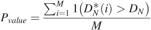 (2.69)


Replacing DN∗DN by WN2∗WN2,AN2∗AN2,UN2∗UN2,LN∗LN
 in Equation (2.69), we can simulate the P-values for other statistics.
From common practice, we may set αlevel = 0.05αlevel=0.05, which means the hypothesized parametric univariate distribution cannot be rejected if Pvalue ≥ 0.05 = αlevelPvalue≥0.05=αlevel. Furthermore, the larger the M, the closer the simulated P-value to its true P-value.
Example 2.8 Using the observed annual peak streamflow given in Table 2.1, compute the goodness-of-fit with the use of KS, CM, AD, modified weighted Watson, Liao, and Shimokawa tests, given the gamma distribution as the tested probability distribution.
Table 2.1. Observed annual peak streamflow.
| No. | Peak (cfs) | No. | Peak (cfs) |
|---|---|---|---|
| 1 | 2,300 | 26 | 4,730 |
| 2 | 3,390 | 27 | 1,060 |
| 3 | 1,710 | 28 | 3,290 |
| 4 | 9,780 | 29 | 7,880 |
| 5 | 10,500 | 30 | 13,800 |
| 6 | 13,700 | 31 | 10,500 |
| 7 | 6,500 | 32 | 7,150 |
| 8 | 3,710 | 33 | 1,030 |
| 9 | 536 | 34 | 13,100 |
| 10 | 17,000 | 35 | 2,920 |
| 11 | 6,630 | 36 | 5,210 |
| 12 | 1,220 | 37 | 4,460 |
| 13 | 4,980 | 38 | 3,100 |
| 14 | 2,840 | 39 | 1,520 |
| 15 | 3,220 | 40 | 29,800 |
| 16 | 2,440 | 41 | 2,740 |
| 17 | 1,320 | 42 | 1,740 |
| 18 | 16,000 | 43 | 557 |
| 19 | 16,100 | 44 | 5,350 |
| 20 | 1,180 | 45 | 11,200 |
| 21 | 5,440 | 46 | 4,930 |
| 22 | 2,420 | 47 | 3,490 |
| 23 | 9,140 | 48 | 2,990 |
| 24 | 6,700 | 49 | 6,160 |
| 25 | 912 | 50 | 1,480 |
| 51 | 496 |
Solution:
Gamma distribution is given as follows:

Following the test procedures given previously, the following steps are needed for the goodness-of-fit test calculations.
Step 1: Order the streamflow values in increasing order and estimate the parameters for the probability distribution (as shown in Table 2.2). In Table 2.2, the parameters of gamma distribution are estimated using the MLE.
Table 2.2. Ordered annual peak streamflow and parameter estimated with MLE.
| Order | Peak (cfs) | Order | Peak (cfs) |
|---|---|---|---|
| 1 | 496 | 26 | 3,710 |
| 2 | 536 | 27 | 4,460 |
| 3 | 557 | 28 | 4,730 |
| 4 | 912 | 29 | 4,930 |
| 5 | 1,030 | 30 | 4,980 |
| 6 | 1,060 | 31 | 5,210 |
| 7 | 1,180 | 32 | 5,350 |
| 8 | 1,220 | 33 | 5,440 |
| 9 | 1,320 | 34 | 6,160 |
| 10 | 1,480 | 35 | 6,500 |
| 11 | 1,520 | 36 | 6,630 |
| 12 | 1,710 | 37 | 6,700 |
| 13 | 1,740 | 38 | 7,150 |
| 14 | 2,300 | 39 | 7,880 |
| 15 | 2,420 | 40 | 9,140 |
| 16 | 2,440 | 41 | 9,780 |
| 17 | 2,740 | 42 | 10,500 |
| 18 | 2,840 | 43 | 10,500 |
| 19 | 2,920 | 44 | 11,200 |
| 20 | 2,990 | 45 | 13,100 |
| 21 | 3,100 | 46 | 13,700 |
| 22 | 3,220 | 47 | 13,800 |
| 23 | 3,290 | 48 | 16,000 |
| 24 | 3,390 | 49 | 16,100 |
| 25 | 3,490 | 50 | 17,000 |
| 51 | 29,800 | ||
| Parameters: α = 1.3164, β = 4.4737 × 10³. | |||
Step 2: Compute the corresponding test statistics:
1. Table 2.3 lists the CDF computed from increasingly ordered annual peak streamflow data for the fitted gamma distribution.
2. Compute the test statistics. The computation example is using Q(1) = 496 cubic feet per second (cfs) for a sample size of N = 51. The full list of the computation is given in Table 2.3.
KS test (DNDN) (Equation (2.64)), the distance for i = 1 is computed as follows:
δ̂1=max1N−Fx1Fx1−1−1N=max159−0.04410.0441−0=0.0441
CM test (WN2
 ) (Equation (2.65)): the quantity inside of summation (i.e., CMdi) for I = 1 is computed as follows:
CMd1=Fx1−21−12N2=0.0441−12512=0.0012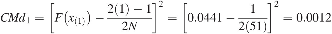
AD test (AN2
 ) (Equation (2.66)): the quantity inside of the summation (i.e., ADdi) for i = 1 is computed as follows:
ADd1 = (2(1) − 1) ln (F(x(1)(1 − F(x(1))) = ln (0.0441(1 − 0.0441)) = − 3.1670ADd1=21−1ln(F(x11−Fx1=ln0.04411−0.0441=−3.1670
Modified weighted Watson test (UN2)
 (Equation (2.67)): the quantity inside of the summation for i = 1 is computed as follows:
d1=Fx1−1N+11N−1+1=0.0441−15251=0.0035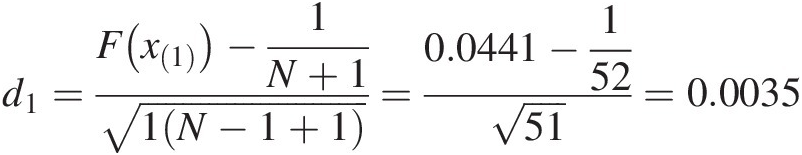
Liao and Shimokawa test (LN)LN) (Equation (2.68)): the quantity inside of the summation (i.e., Ldi) for i = 1 is computed as follows:
Ld1=max1N−Fx1Fx1−1−1NF(x1)(1−Fx1=max151−0.04410.04410.04411−0.0441=0.2147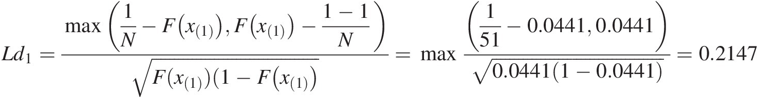
Now, substituting the quantities computed in Table 2.3 back into Equations (2.64)–(2.68), we can calculate the final test statistics for each goodness-of-fit test as follows:
KS test: DN = 0.0883DN=0.0883
CM test: WN2=0.0558
AD test: AN2=0.3534
Modified weighted Watson test: UN2=0.2993
Liao and Shimokawa test: LN = 5.1695LN=5.1695
3. Apply the parametric bootstrap method M times to approximate the P-value with given significance level α. Here we choose M = 1,000 and α = 0.05. To illustrate the procedure, we will use one parametric bootstrap simulation as an example:
a. Generate IID streamflow from the fitted gamma distribution (with parameters given in Table 2.2 of sample size N = 51), and sort the simulated streamflow values in increasing order (Table 2.4).
b. Reestimate the parameters of gamma distribution and calculate the CDF and corresponding test statistics using the simulated streamflow. We have discussed how to compute the test statistics previously (steps 1 and 2), here we will only present the final results:
i. Estimated parameters: α1∗=1.3241,β1∗=4.8206×10³
 .
.
ii. Test statistics computed from simulated streamflow with reestimated parameters:
DN1∗=0.1400;WN12∗=0.1496;AN12∗=0.8237;UN12∗=0.6595;LN1∗=6.8445.
c. Repeat the parametric bootstrap simulation 1,000 times. We can approximate the P-value and corresponding critical value using the KS test as an example:
P-value=∑i=1M1DNi∗>DNM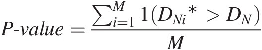
The critical value can be approximated by interpolation from computed DNi∗,i=1,…,M
 and its empirical distribution.
KS test final result:
DN = 0.0883, P = 0.222, Crivalue = 0.1156DN=0.0883,P=0.222,Crivalue=0.1156.
CM test final results:
WN2=0.0558,P=0.456,Crivalue=0.1327.
AD test final results:
AN2=0.3534,P=0.489,Crivalue=0.7549.
Modified weighted Watson test final results:
UN2=0.2993,P=0.532,Crivalue=0.6821.
Liao and Shimokawa test final results:
LN = 5.1695, P = 0.438, Crivalue = 6.9574LN=5.1695,P=0.438,Crivalue=6.9574.


Table 2.3. CDF and corresponding statistics computed for the ordered annual peak streamflow.
| Order | Peak (cfs) | CDF | Test statistics | ||||
|---|---|---|---|---|---|---|---|
KS δî | CM (CMdi)CMdi | AD (ADdi)ADdi | UN2 (di)di (di)di | LNLN (Ldi)Ldi | |||
| 1 | 496 | 0.0441 | 0.0441 | 0.0012 | –9.0297 | 0.0035 | 0.2147 |
| 2 | 536 | 0.0486 | 0.0290 | 0.0004 | –18.6652 | 0.0010 | 0.1347 |
| 3 | 557 | 0.0510 | 0.0117 | 3.73E-06 | –29.9324 | –0.0006 | 0.0534 |
| 4 | 912 | 0.0933 | 0.0345 | 0.0006 | –37.5253 | 0.0012 | 0.1185 |
| 5 | 1,030 | 0.1079 | 0.0295 | 0.0004 | –42.8437 | 0.0008 | 0.0950 |
| 6 | 1,060 | 0.1117 | 0.0136 | 1.46E-05 | –51.7633 | –0.0002 | 0.0433 |
| 7 | 1,180 | 0.1267 | 0.0105 | 5.38E-07 | –57.9304 | –0.0004 | 0.0317 |
| 8 | 1,220 | 0.1318 | 0.0251 | 0.0002 | –60.4520 | –0.0012 | 0.0742 |
| 9 | 1,320 | 0.1444 | 0.0321 | 0.0005 | –64.5542 | –0.0015 | 0.0913 |
| 10 | 1,480 | 0.1646 | 0.0315 | 0.0005 | –69.6576 | –0.0014 | 0.0849 |
| 11 | 1,520 | 0.1697 | 0.0460 | 0.0013 | –73.3189 | –0.0020 | 0.1226 |
| 12 | 1,710 | 0.1936 | 0.0417 | 0.0010 | –74.3267 | –0.0017 | 0.1055 |
| 13 | 1,740 | 0.1974 | 0.0575 | 0.0023 | –74.0839 | –0.0023 | 0.1445 |
| 14 | 2,300 | 0.2665 | 0.0116 | 3.37E-06 | –68.0529 | –0.0001 | 0.0263 |
| 15 | 2,420 | 0.2810 | 0.0131 | 1.11E-05 | –69.0385 | –0.0003 | 0.0292 |
| 16 | 2,440 | 0.2834 | 0.0304 | 0.0004 | –73.1189 | –0.0010 | 0.0674 |
| 17 | 2,740 | 0.3187 | 0.0146 | 2.34E-05 | –73.1350 | –0.0003 | 0.0314 |
| 18 | 2,840 | 0.3302 | 0.0227 | 0.0002 | –74.0442 | –0.0006 | 0.0483 |
| 19 | 2,920 | 0.3393 | 0.0332 | 0.0005 | –72.2151 | –0.0010 | 0.0701 |
| 20 | 2,990 | 0.3473 | 0.0449 | 0.0012 | –74.5592 | –0.0015 | 0.0943 |
| 21 | 3,100 | 0.3596 | 0.0522 | 0.0018 | –75.8782 | –0.0017 | 0.1087 |
| 22 | 3,220 | 0.3728 | 0.0585 | 0.0024 | –76.1786 | –0.0020 | 0.1211 |
| 23 | 3,290 | 0.3805 | 0.0705 | 0.0037 | –78.3911 | –0.0024 | 0.1452 |
| 24 | 3,390 | 0.3913 | 0.0793 | 0.0048 | –78.8187 | –0.0027 | 0.1626 |
| 25 | 3,490 | 0.4019 | 0.0883 | 0.0062 | –78.4213 | –0.0030 | 0.1801 |
| 26 | 3,710 | 0.4248 | 0.0850 | 0.0056 | –71.8666 | –0.0029 | 0.1719 |
| 27 | 4,460 | 0.4979 | 0.0315 | 0.0005 | –64.2055 | –0.0008 | 0.0631 |
| 28 | 4,730 | 0.5222 | 0.0268 | 0.0003 | –63.0316 | –0.0006 | 0.0537 |
| 29 | 4,930 | 0.5396 | 0.0290 | 0.0004 | –62.4556 | –0.0007 | 0.0582 |
| 30 | 4,980 | 0.5439 | 0.0444 | 0.0012 | –63.4603 | –0.0013 | 0.0891 |
| 31 | 5,210 | 0.5630 | 0.0448 | 0.0012 | –62.2242 | –0.0013 | 0.0904 |
| 32 | 5,350 | 0.5743 | 0.0531 | 0.0019 | –61.8107 | –0.0016 | 0.1074 |
| 33 | 5,440 | 0.5815 | 0.0656 | 0.0031 | –62.1859 | –0.0021 | 0.1329 |
| 34 | 6,160 | 0.6349 | 0.0318 | 0.0005 | –57.2926 | –0.0008 | 0.0660 |
| 35 | 6,500 | 0.6579 | 0.0284 | 0.0003 | –55.3675 | –0.0006 | 0.0598 |
| 36 | 6,630 | 0.6664 | 0.0395 | 0.0009 | –52.4782 | –0.0011 | 0.0838 |
| 37 | 6,700 | 0.6708 | 0.0547 | 0.0020 | –53.2252 | –0.0017 | 0.1163 |
| 38 | 7,150 | 0.6983 | 0.0468 | 0.0014 | –50.1841 | –0.0014 | 0.1020 |
| 39 | 7,880 | 0.7383 | 0.0264 | 0.0003 | –40.2878 | –0.0005 | 0.0600 |
| 40 | 9,140 | 0.7960 | 0.0313 | 0.0005 | –35.0231 | 0.0012 | 0.0777 |
| 41 | 9,780 | 0.8205 | 0.0362 | 0.0007 | –31.0876 | 0.0015 | 0.0942 |
| 42 | 10,500 | 0.8446 | 0.0407 | 0.0010 | –28.9422 | 0.0018 | 0.1124 |
| 43 | 10,500 | 0.8446 | 0.0211 | 0.0001 | –27.6059 | 0.0009 | 0.0583 |
| 44 | 11,200 | 0.8651 | 0.0220 | 0.0001 | –24.8973 | 0.0010 | 0.0643 |
| 45 | 13,100 | 0.9084 | 0.0457 | 0.0013 | –20.6088 | 0.0024 | 0.1583 |
| 46 | 13,700 | 0.9190 | 0.0367 | 0.0007 | –18.4602 | 0.0021 | 0.1344 |
| 47 | 13,800 | 0.9207 | 0.0187 | 7.92E-05 | –18.3082 | 0.0011 | 0.0692 |
| 48 | 16,000 | 0.9497 | 0.0281 | 0.0003 | –14.2122 | 0.0019 | 0.1284 |
| 49 | 16,100 | 0.9507 | 0.0101 | 8.56E-08 | –9.9778 | 0.0007 | 0.0466 |
| 50 | 17,000 | 0.9591 | 0.0213 | 0.0001 | –9.0618 | –0.0002 | 0.1075 |
| 51 | 29,800 | 0.9973 | 0.0169 | 5.02E-05 | –4.8272 | 0.0023 | 0.3244 |
Table 2.4. Generating gamma distributed streamflows and sorting in increasing order.
| No. | Generated | Order | Sorted |
|---|---|---|---|
| 1 | 8,683.20 | 1 | 51.56 |
| 2 | 921.76 | 2 | 127.24 |
| 3 | 7,874.64 | 3 | 574.63 |
| 4 | 10,470.50 | 4 | 766.02 |
| 5 | 3,019.36 | 5 | 872.26 |
| 6 | 5,625.04 | 6 | 921.76 |
| 7 | 1,548.26 | 7 | 1,317.86 |
| 8 | 7,719.17 | 8 | 1,411.29 |
| 9 | 15,787.45 | 9 | 1,548.26 |
| 10 | 1,592.99 | 10 | 1,592.99 |
| 11 | 19,530.55 | 11 | 2,007.60 |
| 12 | 12,160.63 | 12 | 2,193.47 |
| 13 | 1,411.29 | 13 | 2,194.08 |
| 14 | 13,026.83 | 14 | 2,431.96 |
| 15 | 8,385.82 | 15 | 2,801.57 |
| 16 | 3,906.03 | 16 | 3,019.36 |
| 17 | 9,190.72 | 17 | 3,282.55 |
| 18 | 8,067.79 | 18 | 3,643.24 |
| 19 | 8,948.61 | 19 | 3,752.08 |
| 20 | 11,060.80 | 20 | 3,906.03 |
| 21 | 2,431.96 | 21 | 4,003.93 |
| 22 | 1,317.86 | 22 | 4,407.35 |
| 23 | 2,194.08 | 23 | 4,895.35 |
| 24 | 5,589.25 | 24 | 5,589.25 |
| 25 | 3,643.24 | 25 | 5,625.04 |
| 26 | 1,2416.01 | 26 | 6,351.30 |
| 27 | 872.26 | 27 | 6,756.52 |
| 28 | 4,003.93 | 28 | 7,025.33 |
| 29 | 3,752.08 | 29 | 7,581.81 |
| 30 | 6,756.52 | 30 | 7,719.17 |
| 31 | 12,419.87 | 31 | 7,789.85 |
| 32 | 9,953.94 | 32 | 7,874.64 |
| 33 | 10,547.60 | 33 | 8,067.79 |
| 34 | 4,895.35 | 34 | 8,329.23 |
| 35 | 13,512.85 | 35 | 8,385.82 |
| 36 | 2,193.47 | 36 | 8,683.20 |
| 37 | 51.56 | 37 | 8,872.19 |
| 38 | 7,025.33 | 38 | 8,948.61 |
| 39 | 574.63 | 39 | 9,190.72 |
| 40 | 8,329.23 | 40 | 9,953.94 |
| 41 | 4,407.35 | 41 | 10,131.30 |
| 42 | 7,581.81 | 42 | 10,470.50 |
| 43 | 127.24 | 43 | 10,547.60 |
| 44 | 2,801.57 | 44 | 11,060.80 |
| 45 | 7,789.85 | 45 | 12,160.63 |
| 46 | 2,007.60 | 46 | 12,416.01 |
| 47 | 766.02 | 47 | 12,419.87 |
| 48 | 10,131.30 | 48 | 13,026.83 |
| 49 | 6,351.30 | 49 | 13,512.85 |
| 50 | 8,872.19 | 50 | 15,787.45 |
| 51 | 3,282.55 | 51 | 19,530.55 |
Chi-Square Goodness-of-Fit Test
Rather than measuring the difference between the empirical CDF and the fitted parametric CDF, the chi-square goodness-of-fit test deals with the frequency directly. As its name indicates, the limiting distribution is the chi-square distribution with its statistic expressed as follows:
 (2.70)
In Equation (2.70), oioi is the observed frequency count for the level-i of a variable; eiei is the corresponding expected frequency count from the fitted probability distribution; K is the number of levels of the random variable; m is the number of the parameters of the fitted probability distribution, and K-m-1 is the degree of freedom of the limiting chi-square distribution. In other words, Equation (2.70) is actually comparing the relative frequency computed from a histogram with K-bins to the fitted parametric distribution, i.e., (1) level-i is equivalent to the bin-i of the histogram and (2) number of level K is equivalent to the total number of bins (K) of the histogram.
The simplest rule of thumb to determine the number of bins for a histogram is given as follows:
Example 2.9 Rework Example 2.8 with the chi-square goodness-of-fit test.
Solution:
Step 1: To apply the chi-square goodness-of-fit study, we will first study the frequency histogram.
Applying Equation (2.71), we obtain the number of bins for the frequency histogram as follows:
k = ⌈1 + log251⌉ = 7k=1+log251=7. The observed relative frequency is shown in Figure 2.1 and Table 2.5.

Figure 2.1 Relative frequency plot.
Table 2.5. Relative frequency and corresponding data range.
| Relative frequency (observed) | Data interval | Estimated frequency computed from fitted gamma distribution |
|---|---|---|
| 0.5294 | [496, 4682.2857] | 0.4739 |
| 0.2353 | [4682.2857, 8868.5714] | 0.2667 |
| 0.0980 | [8868.5714, 13054.8571] | 0.1228 |
| 0.1176 | [13054.8571, 17241.1429] | 0.0536 |
| 0 | [17241.1429, 21427.4286] | 0.0227 |
| 0 | [21427.4286, 25613.7143] | 0.0095 |
| 0.0196 | [25613.7143, 29800] | 0.0039 |
Step 2: Compute the estimated frequency with the fitted gamma distribution (parameters listed in Table 2.2) to compute the frequency of the corresponding data interval in Table 2.5). Using data interval of [496, 4682.2857], we have the following:
The rest of the results are listed in Table 2.5.
Step 3: Computing test statistics using Equation (2.70), we have the following:
From the chi-square goodness-of-fit, we know the test statistics should follow the chi-square distribution with the degree of freedom, i.e., d. o. f. = K − m − 1 = 7 − 2 − 1 = 4d.o.f.=K−m−1=7−2−1=4.
Choosing the significance level α = 0.05α=0.05, we can calculate the corresponding critical value as follows:

2.4.2 Goodness-of-Fit Measures for Bivariate Probability Distributions
In this section, we briefly discuss two popular goodness-of-fit measures, both of which are based on the Rosenblatt transform (Rosenblatt, 1952). The Rosenblatt transform states that a bivariate random variable Z = [X, Y]Z=XY may be modeled by the fitted joint distribution function of F̂X,Yxy;θ̂ . Let
. Let
 (2.72)
Based on the Bayes theorem, the joint distribution function F̂X,Yxy may be expressed as follows:
 (2.73)
In Equations (2.72) and (2.73), T1, T2T1,T2 are independent and following a uniform distribution; F̂Xx is the fitted distribution of random variable X; and F̂Y∣X=x
 is the conditional distribution derived from the fitted joint distribution F̂X,Yxy
 and the fitted univariate distribution F̂Xx
 .
.
Chi-Square Goodness-of-Fit Test
As stated in Rosenblatt (1952), the chi-square goodness-of-fit test for the univariate distribution can be extended to evaluate the goodness-of-fit for the multivariate distribution. The null hypothesis T = [T1, T2]T=T1T2 is from the distribution on a unit square [0, 1]2012, if the hypothesized joint distribution is proper. Dividing the unite square into N2 cells, the chi-square test may be generated as follows (Rosenblatt, 1952):
i. Define cell Cj1, j2Cj1,j2 as:
Cj1,j2=TjiN<ti<ji+1Ni=12where j1, j2 ∈ [0, …, N − 1]j1,j2∈0…N−1, with each cell having the same probability mass as 1/N21/N2.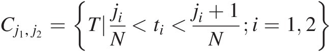 (2.74)
ii. Let vj1, j2vj1,j2 be the number of TiTi in cell Cj1, j2Cj1,j2, the chi-square test statistics may be calculated to evaluate whether Z = [X, Y]Z=XY may be drawn from the fitted distribution F̂X,Yxyθ̂
 using the following:
χ2=∑i=1nvj1,j2−nN22nN2The test statistic computed using Equation (2.75) should follow the chi-square distribution with the degrees of freedom of (N − 1)2N−12.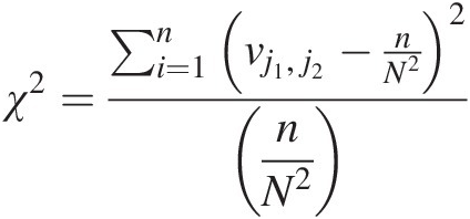 (2.75)


Bivariate (Multivariate) KS Goodness-of-Fit Test
As with the univariate KS goodness-of-fit test, the bivariate KS goodness-of-fit test measures the distance of empirical joint distribution Fn(x, y)Fnxy from its true joint distribution FX, Y(x, y)FX,Yxy, expressed as follows:
Applying the Rosenblatt transform to the fitted joint distribution (i.e., Equations (2.72) and (2.73)), the test of Equation (2.76) is equivalent to the following test:
where GnGn is the empirical distribution of the transformed variables.
Given T1, T2T1,T2 being independent random variables, the null hypothesis of FX,Y=F̂X,Y(x,y;θ̂ ) is equivalent to that of FT1, T2 = T1 ⊥ T2 = Π(T1, T2)FT1,T2=T1⊥T2=ΠT1T2.
To assess Equation (2.77), Justel et al. (1994) proposed the permutation method. One may also apply the same parametric bootstrap method as that for univariate analysis to approximate the P-value of the test statistic discussed for the univariate goodness-of-fit test.
Example 2.10 Assess the goodness-of-fit for the bivariate data listed in Table 2.6, given that the data may be modeled with bivariate normal distribution (true population mean and population covariance matrix given asfollows:μ=[1001000];COV=[4005605601600]).

Table 2.6. Bivariate sample dataset.
| No. | X | Y | No. | X | Y |
|---|---|---|---|---|---|
| 1 | 119 | 1,033 | 26 | 106 | 1,034 |
| 2 | 106 | 1,021 | 27 | 95 | 993 |
| 3 | 103 | 993 | 28 | 109 | 1,011 |
| 4 | 110 | 1,008 | 29 | 108 | 1,037 |
| 5 | 105 | 1,065 | 30 | 75 | 982 |
| 6 | 81 | 909 | 31 | 81 | 983 |
| 7 | 97 | 1,059 | 32 | 85 | 1,015 |
| 8 | 97 | 1,006 | 33 | 90 | 1,012 |
| 9 | 89 | 1,014 | 34 | 94 | 998 |
| 10 | 134 | 1,000 | 35 | 100 | 981 |
| 11 | 82 | 959 | 36 | 39 | 897 |
| 12 | 90 | 979 | 37 | 91 | 1,021 |
| 13 | 86 | 992 | 38 | 125 | 989 |
| 14 | 77 | 919 | 39 | 79 | 969 |
| 15 | 96 | 1,008 | 40 | 119 | 970 |
| 16 | 95 | 958 | 41 | 107 | 1,039 |
| 17 | 131 | 1,045 | 42 | 99 | 1,024 |
| 18 | 95 | 1,012 | 43 | 104 | 1,005 |
| 19 | 79 | 980 | 44 | 69 | 954 |
| 20 | 132 | 1,076 | 45 | 98 | 927 |
| 21 | 125 | 1,063 | 46 | 132 | 1,062 |
| 22 | 95 | 975 | 47 | 102 | 940 |
| 23 | 70 | 965 | 48 | 101 | 935 |
| 24 | 91 | 961 | 49 | 85 | 982 |
| 25 | 97 | 958 | 50 | 99 | 972 |
Solution: Applying the Rosenblatt transform (Equations (2.72) and (2.73)), we can compute T1 and T2 directly from the fitted bivariate normal distribution as follows:
 (2.78a)
 (2.78b)
Table 2.7 lists the estimated T̂1,T̂2 from Equations (2.78a) and (2.78b).
Table 2.7. Estimated T̂1,T̂2 from the bivariate normal distribution.

| X | T̂1 | Y | T̂2 | X | T̂1 | Y | T̂2 |
|---|---|---|---|---|---|---|---|
| 119 | 0.829 | 1,033 | 0.589 | 106 | 0.618 | 1,034 | 0.815 |
| 106 | 0.618 | 1,021 | 0.670 | 95 | 0.401 | 993 | 0.500 |
| 103 | 0.560 | 993 | 0.348 | 109 | 0.674 | 1,011 | 0.478 |
| 110 | 0.691 | 1,008 | 0.417 | 108 | 0.655 | 1,037 | 0.817 |
| 105 | 0.599 | 1,065 | 0.979 | 75 | 0.106 | 982 | 0.724 |
| 81 | 0.171 | 909 | 0.012 | 81 | 0.171 | 983 | 0.632 |
| 97 | 0.440 | 1,059 | 0.987 | 85 | 0.227 | 1,015 | 0.896 |
| 97 | 0.440 | 1,006 | 0.639 | 90 | 0.309 | 1,012 | 0.819 |
| 89 | 0.291 | 1,014 | 0.848 | 94 | 0.382 | 998 | 0.589 |
| 134 | 0.955 | 1,000 | 0.048 | 100 | 0.500 | 981 | 0.253 |
| 82 | 0.184 | 959 | 0.290 | 39 | 0.001 | 897 | 0.269 |
| 90 | 0.309 | 979 | 0.403 | 91 | 0.326 | 1,021 | 0.880 |
| 86 | 0.242 | 992 | 0.658 | 125 | 0.894 | 989 | 0.054 |
| 77 | 0.125 | 919 | 0.044 | 79 | 0.147 | 969 | 0.478 |
| 96 | 0.421 | 1,008 | 0.683 | 119 | 0.829 | 970 | 0.024 |
| 95 | 0.401 | 958 | 0.110 | 107 | 0.637 | 1,039 | 0.847 |
| 131 | 0.939 | 1,045 | 0.522 | 99 | 0.480 | 1,024 | 0.813 |
| 95 | 0.401 | 1,012 | 0.747 | 104 | 0.579 | 1,005 | 0.492 |
| 79 | 0.147 | 980 | 0.629 | 69 | 0.061 | 954 | 0.464 |
| 132 | 0.945 | 1,076 | 0.863 | 98 | 0.460 | 927 | 0.007 |
| 125 | 0.894 | 1,063 | 0.837 | 132 | 0.945 | 1,062 | 0.726 |
| 95 | 0.401 | 975 | 0.264 | 102 | 0.540 | 940 | 0.014 |
| 70 | 0.067 | 965 | 0.597 | 101 | 0.520 | 935 | 0.010 |
| 91 | 0.326 | 961 | 0.178 | 85 | 0.227 | 982 | 0.542 |
| 97 | 0.440 | 958 | 0.093 | 99 | 0.480 | 972 | 0.176 |
Chi-Square Test
Applying Equation (2.74), Table 2.8 lists the numbers that fulfill the condition. Here N = 6 is chosen for the number of bins for both random variables X and Y. Applying Equation (2.75), we compute the chi-square test statistics as follows: χtest2=26.64 .
.
With the chi-square distribution as the limiting distribution (d.f. = 25), we compute the critical value from the chi-square distribution with a significance level of α = 0.05α=0.05 as χcri2=37.65 . We obtain χtest2<χcri2
 . Equivalently, we compute the P-value of the test statistics as follows:

Thus, we reach the conclusion that the sample dataset listed in Table 2.6 may be modeled with the true population parameters.
Table 2.8. Pairs of (T̂1,T̂2 ) within each interval.

| [0, 1/6] | [1/6, 1/3] | [1/3, 1/2] | [1/2, 2/3] | [2/3, 5/6] | [5/6, 1] | |
|---|---|---|---|---|---|---|
| [0, 1/6] | 1 | 1 | 2 | 2 | 1 | 0 |
| [1/6, 1/3] | 1 | 2 | 1 | 3 | 1 | 3 |
| [1/3, 1/2] | 3 | 3 | 1 | 3 | 3 | 1 |
| [1/2, 2/3] | 2 | 1 | 2 | 0 | 3 | 2 |
| [2/3, 5/6] | 1 | 0 | 2 | 1 | 0 | 0 |
| [5/6, 1] | 2 | 0 | 0 | 1 | 1 | 2 |
Bivariate KS goodness-of-fit test
To apply the bivariate KS goodness-of-fit test, the hypothesis is that the variables (T1, T2T1,T2) after Rosenblatt transformation are independent. This implies the joint distribution of T1, T2T1,T2 may be simply expressed as F = T1T2F=T1T2. The KS statistic is computed by comparing the empirical joint distribution of T1, T2T1,T2 with the hypothesized independence assumption.
Similar to the univariate goodness-of-fit test, the KS test statistics is evaluated as Dn = 0.1684Dn=0.1684. With parametric bootstrap simulation (N = 5,000), we obtain the corresponding P-value as P-value = 0.3140.
Both bivariate chi-square and KS goodness-of-fit tests suggest the data given in Table 2.6 may be sampled from the true population.
2.5 Quantile Estimation
In flood frequency analysis, the return period (T) of a given flood magnitude, called quantile, or the flood magnitude corresponding to a given return is needed. The return period is related to the probability of nonexceedance (F) as
 (2.78)
where F = F(xT)F=FxT, where xTxT (quantile) corresponds to T, that is, the probability of a flood of magnitude smaller than or equal to xTxT. If the CDF of a distribution can be expressed as explicitly in closed form, then xTxT can be determined directly. Otherwise, it has to be computed numerically. Chow (1954) proposed a general formula for computing xTxT as
(2.78a)where KTKT is the frequency factor, which is a function of the return period and the distribution parameters, and x¯ and σ are the mean and standard deviation of the distribution respectively. Chow (1964) has given KTKT for different frequency distributions. For the normal distribution, it equals the standard normal variate.
2.6 Confidence Intervals
When estimating the quantile of a given return period, it is important to provide an estimate of the accuracy of the estimate. The accuracy of the estimate depends on the distribution parameters (method of parameter estimation), sample size, and dependence or independence of observed data. The variability of estimated value is measured by the standard error of estimate, which will depend on the distribution in use. There have been many studies that have computed the standard error of estimate of quantile for different distributions. It considers the error due to small sample size but not the error due to the use of an inappropriate distribution. Cunnane (1989) defined the standard error of estimate sTsT of xTxT as
 (2.79)
where E is the expectation operator. Since sTsT varies with the parameter estimation method, each method has its own standard error of estimate, so the method yielding the smallest error is considered the most efficient method. If the sample size n tends to infinity, then the distribution of xTxT is asymptotically normal with mean xT¯ and variance sT2
 . Then, an approximate confidence interval (1−α) for xTxT can be expressed as
 (2.79a)
where t is the standard normal variate. Methods for computing confidence intervals for skewed distributions are available (USWRC, 1981).
2.7 Bias and Root Mean Square Error (RMSE) of Parameter Estimates
Let θθ and θ̂ be the true and estimated parameter of a probability distribution respectively. The bias of the θ̂
 with respect to θθ is defined as follows:
 (2.80a)
In Equation (2.80a), the estimates are unbiased if the bias = 0.
In a similar vein, the RMSE of θ̂ with respect to θθ is defined as follows:
 (2.80b)
Equation (2.80b) becomes the standard deviation of the estimator, if the estimator is unbiased.
2.8 Risk Analysis
In general, the probabilistic risk assessment and analysis are composed of two key components: (1) the severity of the possible consequence; and (2) the likelihood (probability) associated with the consequence. In other words, risk may be represented by the probability of loss ranging from [0, 1].
In water resources engineering, risk is one key component to the analysis of extreme events. Conveniently, the return period (i.e., univariate/multivariate) has been applied to represent risk. For example, the annual maximum discharge event with a 100-year return period (i.e., P(Q>q) = 0.01PQ>q=0.01), representing the risk of the occurrence of peak discharge roughly about once a 100 year, is commonly used to design the designated infrastructure, such as a levee. The probable maximum precipitation (PMP) is required to analyze classified dams. For urban hydrology, storm events for a given return period are applied for highway drainage design (with different highway categories) and storm sewer (or combined sewer) design. In what follows, the concept of risk, through return period, is briefly reviewed for both univariate and multivariate cases.
2.8.1 Univariate Risk Analysis through Return Period
As discussed previously, the univariate risk may be expressed as the probability of the occurrence of the event of certain magnitude. With the assumption of continuous univariate variable, the risk may be represented as P(X>x∗)PX>x∗. For the univariate sequence (i.e., annual sequence or partial duration sequence) under the stationary assumption, the return period of X>x∗X>x∗ is given as follows:
 (2.81)
where μμ denotes the average interarrival time between two events (or realizations of the process); n denotes the length of time duration; m denotes the number of events (or realizations) of n length of time durations; x∗x∗ denotes the design value (or critical value); and F denotes the probability distribution function of X.
The probability that a value of X, x, will occur in n successive years can be given by 1−1Tn . Hence, the probability that x will occur for the first time in n years can be expressed as 1T1−1Tn−1
 .
.
The probability that the value will occur at least once in n years can be given as
 (2.82)
Here R can be called risk. Equation (2.82) can be used to compute the probability that x will occur within its return period:
 (2.83)
If T is large, then
For practical applications, one can compute the values of T for different values of R and n.
2.8.2 Bivariate (Multivariate) Risk Analysis through Return Period
Unlike with the univariate risk analysis, one may select different scenarios for the bivariate (multivariate) risk analysis. Here, we will present the return period for the bivariate case only. Let random variables {X, Y} with the marginal and joint distributions be denoted as FX(x), FY(y), FX, Y(x, y)FXx,FYy,FX,Yxy, and we immediately have the univariate return period from Equation (2.81) as follows:
 (2.84)
Following Shiau (2003), the bivariate risk analysis may be evaluated through (1) an “OR” case (X ≥ x ∪ Y ≥ yX≥x∪Y≥y); (2) an “AND” case (X ≥ x ∩ Y ≤ y)X≥x∩Y≤y); and (3) a “CONDITIONAL” case (X ≥ x|Y ≥ y; or Y ≥ y|X ≥ x)X≥xY≥yorY≥yX≥x). In what follows, each case is further discussed.
“OR” Case (X ≥ x ∪ Y ≥ y);X≥x∪Y≥y
The risk of “OR” case can be expressed as the likelihood (probability) of either event X: X ≥ xX≥x or event Y: Y ≥ yY≥y, i.e., P(X ≥ x ∪ Y ≥ y)PX≥x∪Y≥y. This probability can be written as follows:
The risk expressed through the return period of the “OR” case can then be given as follows:
 (2.86)
“AND” Case: (X ≥ x ∩ Y ≥ yX≥x∩Y≥y)
The risk for the “AND” case can be expressed as the likelihood (probability) of both events X and Y that exceed the given magnitude x, yx,y, i.e., P(X ≥ x ∩ Y ≥ y)PX≥x∩Y≥y. This probability can be written as follows:
The risk expressed through the return period of the “AND” case can be given as follows:
 (2.88)
“CONDITIONAL” Case
With the knowledge of event Y exceeding the magnitude of y, the risk of event X exceeding magnitude of x may be represented as the conditional likelihood (probability) of P(X ≥ x| Y ≥ y)PX≥xY≥y. This probability can be given as follows:
 (2.89)
Equation (2.84) may also be derived through the conditional probability distribution F(x| Y ≥ y)FxY≥y as follows:
 (2.90)
Following Shiau (2003) and Salvadori (2004), the risk expressed through the conditional return period of X ≥ x ∣ Y ≥ yX≥x∣Y≥y can be given as follows:
 (2.91)
Similarly, the conditional return period of Y ≥ y ∣ X ≥ xY≥y∣X≥x can be given as follows:
 (2.92)
In a similar vain, risk analysis may be extended to multivariate (d ≥ 3)d≥3) analysis.