Abstract
The term copula is derived from the Latin verb copulare, meaning “to join together.” In the statistics literature, the idea of a copula can be dated back to the nineteenth century in modeling multivariate non-Gaussian distributions. By formulating a theorem, now called Sklar theorem, Sklar (1959) laid the theoretical foundation for the modern copula theory. In general, copulas couple multivariate distribution functions to their one-dimensional marginal distribution functions, which are uniformly distributed in [0, 1]. In other words, copula functions enable us to represent a multivariate distribution with the use of univariate probability distributions (sometimes simply called marginals, or margins), regardless of their forms or types. In this chapter, we will discuss the general concepts of copulas, including their definition, properties, composition and construction, dependence structure, and tail dependence.
3.1 Definition of Copulas
Based on the Sklar’s theorem definition (Sklar, 1959), a copula has two or more dimensions. Let d be the dimension of a copula. Then, a d-dimensional copula can be defined as a mapping function of [0, 1]d→[0, 1]01d→01, i.e., a multivariate cumulative distribution function can be defined in [0, 1]d01d with standard uniform univariate margins.
Copula has the following properties:
1. Let u = [u1, …, ud], ui = Fi(xi) ∈ [0, 1]u=u1…ud,ui=Fixi∈01, if ui = 0ui=0 for any i ≤ di≤d(at least one coordinate of u equals 0).
C(u1, …, ud) = 0Cu1…ud=0(3.1)
2. C(u) = uiCu=ui, if all the coordinates are equal to 1 except uiui, i.e.,
C(1, 1, …, ui, …, 1, 1) = ui, ∀ i ∈ {1, 2, …, d}, ui ∈ [0, 1]C11…ui…11=ui,∀i∈12…d,ui∈01(3.2)
3. C(u1, …, ud)Cu1…ud is bounded, i.e., 0 ≤ C(u1, …, ud) ≤ 10≤Cu1…ud≤1. This property represents the limit of the cumulative joint distribution, i.e., in the range of [0, 1].
4. C(u1, …, ud)Cu1…ud is d-increasing. This means that the volume of any d-dimensional interval is nonnegative, ∀{(a1, …, ad), (b1, …, bd)} ∈ [0, 1]d∀a1…adb1…bd∈01d, where ai ≤ bi,ai≤bi,
∑i1=12∑i2=12⋯∑i1=12−1i1+i2+…+idCx1i1x2i2…xdid≥0 (3.3)
(3.3)
This property indicates the monotone increasing property of the cumulative probability distribution.
5. For every copula C(u1, …, ud)Cu1…ud and every (u1, …, ud)u1…ud in [0, 1]d01d, the following version of the Fréchet–Hoeffding bounds hold:
W(u1, …, ud) ≤ C(u1, …, ud) ≤ M(u1, …, ud); d ≥ 2Wu1…ud≤Cu1…ud≤Mu1…ud;d≥2(3.4)
where Wu1…ud=max1−d+∑i=1dui0 represents the perfectly negatively dependent random variables; M(u1, …, ud) = min (u1, …, ud)Mu1…ud=minu1…ud represents the perfectly positively dependent random variables.
Here, we will first explain the first two properties using the bivariate flood variables (i.e., peak discharge (Q) and flood volume (V)) as an example. Let Q~FQ(q), V~FV(v)Q~FQq,V~FVv in which FQ ≡ u1, FV ≡ u2FQ≡u1,FV≡u2 represent the probability distribution functions of {Q : Q ≥ Qmin}, {V : V ≥ Vmin}Q:Q≥Qmin,V:V≥Vmin, respectively.
To explain property (1), we set u1 = FQ(q), q>Qminu1=FQq,q>Qmin and u2 = FV(v ≤ Vmin) = 0u2=FVv≤Vmin=0. We have C(u1, 0) = H(Q ≤ q, V ≤ Vmin)Cu10=HQ≤qV≤Vmin. With the joint distribution being nondecreasing, we know the volume of the interval [Qmin, Vmin] × [q, Vmin] = [0, 0] × [u1, 0] ≡ 0QminVmin×qVmin=00×u10≡0 which means when the flood volume is lower than the minimum flood volume, the joint distribution of H(Q ≤ q, V ≤ Vmin) = C(u1, 0) ≡ 0HQ≤qV≤Vmin=Cu10≡0. Similarly, we have the following:
To explain property (2), we will again use the bivariate flood variable (i.e., peak discharge and flood volume) as an example. Based on the probability theory, we have the following:
Example 3.1 Explain and prove the first three copula properties.
Solution: Proof of properties (1) and (2).
Properties (1) and (2) may be explained directly using the Fréchet–Hoeffding bounds.
a. C(u1, …, 0, …, ud) = 0, if ui = 0.Cu1…0…ud=0,ifui=0.
Since copula C(u1, …, ud)Cu1…ud represents the joint cumulative probability distribution of random variables {X1, …, Xd}X1…Xd, from Equation (3.4), we have the following:
From

and
Now we have C(u1, …, ud) = 0, ∃ ui = 0, i ∈ [1, d]Cu1…ud=0,∃ui=0,i∈1d. This proves property (1) with ui = 0ui=0. Similarly, property (1) holds for more than one variable equal to zero.
b. C(u1, …, ud) = ui, ∃ uj = 1 j ∈ [1, d] and j≠iCu1…ud=ui,∃uj=1j∈1dandj≠i
Applying the Fréchet–Hoeffding bounds, we have the following:

Thus, we have C(1, …, 1, ui, 1, …, 1) = uiC1…1ui1…1=ui. This proves property 2.
Proof of property (3): It can be shown that if the copula represents the joint cumulative probability distribution of d-dimensional variables, the limit of copula should be [0, 1]. Property (4), i.e., Fréchet–Hoeffding bounds, further ensures property (3).
Example 3.2 Illustrate a case for d = 2d=2 in Equation (3.3) of property (4).
Solution: For d = 2d=2, we have (a1, a2), (b1, b2) ∈ [0, 1]2a1a2,b1b2∈012 and a1 ≤ a2, b1 ≤ b2a1≤a2,b1≤b2 as shown in Figure 3.1(a):
 (3.5)
(3.5)
Therefore, Equation (3.5) follows:

Example 3.3 Illustrate a case for d = 3d=3 in Equation (3.3) of property (4).
Solution: For d = 3 with {(x, y, z) : (x1, x2), (y1, y2), (z1, z2) ∈ [0, 1]3}d=3withxyz:x1x2y1y2z1z2∈013, where x1 ≤ x2, y1 ≤ y2, z1 ≤ z2x1≤x2,y1≤y2,z1≤z2 as shown in Figure 3.1(b),
 (3.7)
(3.7)and

Using the notation in Figure 3.1(b) in Equation (3.7), we have the following:
As introduced previously, copulas are multivariate distribution functions, and each copula induces a probability measure on [0, 1]d01d. In the bivariate case, C(a1, a2)Ca1a2 can be expressed as a joint probability in the rectangle [0, a1] × [0, a2]0a1×0a2. Thus, Equation (3.6) can be interpreted as follows:
Similarly in the trivaraite case, C(a1, a2, a3)Ca1a2a3 can be expressed as a joint probability measure in the cube of [0, a1] × [0, a2] × [0, a3]0a1×0a2×0a3. Equation (3.8) can be interpreted as follows:
6. Let X1, …, XdX1,…,Xd be random variables with margins F1, …, FdF1,…,Fd and joint distribution function F(x1, …, xd)Fx1…xd and ui = Fi(xi), i = 1, …, dui=Fixi,i=1,…,d. X1, …, XdX1,…,Xd are mutually independent if and only if Fx1…xd=∏i=1dFixi
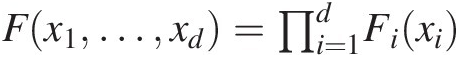 . Copula C(u1, …, ud)Cu1…ud is called the independent or product copula and is defined as follows:
Cu1…ud=∏i=1dui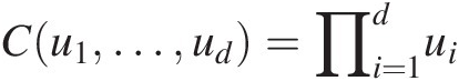 (3.11)


According to Sklar’s theorem, there exists a copula C such that for all x ∈ R : R ∈ (−∞, +∞)x∈R:R∈−∞+∞, the relation between cumulative joint distribution function F(x1, …, xd)Fx1…xd and copula C(u1, …, ud)Cu1…ud can be expressed as follows:
where ui = F(xi) = P(Xi ≤ xi), i = 1, …, d; ui~U(0, 1)ui=Fxi=PXi≤xi,i=1,…,d;ui~U01, if FiFi is continuous. Another way to think about the copula is as follows:
 (3.13)
where xi=Fi−1ui if X is continuous.
Example 3.4 Illustrate Equation (3.12) using the Farlie–Gumbel–Morgenstern (FGM) model.
The FGM model is as follows:
Solution: The joint CDF (JCDF) of the FGM model above can be expressed as follows:
Let u1 = FX(x), u2 = FY(y)u1=FXx,u2=FYy, and we have the following:
The copula captures the essential features of the dependence of bivariate (multivariate) random variables. C is essentially a function that connects the multivariate probability distribution to its marginals. Then the problem of determining H (i.e., the joint cumulative distribution of correlated random variables) reduces to one of determining C. Let c(u1, … , ud)cu1…ud denote the density function of copula C(u1, …, ud)Cu1…ud as follows:
 (3.14a)
The mathematical relation between copula density function c(u1, … , ud)cu1…ud and joint density function f(x1, … , xd)fx1…xd can be expressed as follows:
 (3.14b)
where fi, Fifi,Fi are, respectively, the probability density function and the probability distribution function for random variable XiXi.
Equation (3.14b) may be rewritten as follows:
 (3.14c)
Example 3.5 Using the FGM model in Example 3.4, derive the copula density function and its relation to joint density function.
Solution: From Example 3.4, the FGM model may be represented through the copula function as follows:
C(u1, u2) = u1u2(1 + η(1 − u1)(1 − u2))Cu1u2=u1u21+η1−u11−u2. Then the copula density function can be derived using Equation (3.14a) as follows:
 (3.15a)
The relation between copula density function c(u1, u2)cu1u2 and joint probability density function of the FGM model described in Example 3.4 can be expressed as follows:
where ui = Fi(xi), i = 1, 2ui=Fixi,i=1,2.
As an illustrative example, let X1~ exp (λ)X1~expλ and X2~gamma(α, β)X2~gammaαβ, we may rewrite the probability density function of f(x1, x2)fx1x2 as follows:
 (3.15c)
3.1.1 Bivariate Copula
A bivariate copula C(u1, u2)Cu1u2 is a function from [0, 1] × [0, 1]01×01 into [0,1] to represent the joint cumulative probability distribution function of bivariate random variables with the following properties directly deduced from the discussions earlier as follows:
For every u1, u2u1,u2 in [0, 1]:
1. For every u11 ≤ u12, u21 ≤ u22u11≤u12,u21≤u22 in [0, 1]:
C(u12, u22) − C(u12, u21) − C(u11, u22) + C(u11, u21) ≥ 0Cu12u22−Cu12u21−Cu11u22+Cu11u21≥0(3.17)
Equation (3.17) represents the volume:
 (3.18)
Equation (3.18) represents the second-order derivative of function C(u1, u2)Cu1u2 (Nelsen, 2006). As the representation of the joint distribution of random variables X and Y C(u1, u2) ≡ C(FX(x), FY(y)) ≡ H(x, y)i.e.,Cu1u2≡CFXxFYy≡Hxy, the second-order derivative of C(u1, u2)Cu1u2 represents the copula density function of the bivariate random variable cu1u2=fxyfXxfYy≥0 . This further explains Equations (3.17) and (3.18).
2. When random variables X1X1 and X2X2 are independent, one obtains the so-called product copula:
C(u1, u2) = H(x1, x2) = u1u2, ui = Fi(xi)Cu1u2=Hx1x2=u1u2,ui=Fixi(3.19)
3. For every u1, u2u1,u2 in [0, 1] with the corresponding copula C(u1, u2)Cu1u2, the following Fréchet–Hoeffding bounds hold:
max(u1 + u2 − 1, 0) ≤ C(u, v) ≤ min (u1, u2)maxu1+u2−10≤Cuv≤minu1u2(3.20)
Example 3.6 Express the bivariate Gaussian copula and its density function.
Solution: The bivariate Gaussian copula is a distribution over the unit square [0, 1]2012, which is constructed from the bivariate normal distribution through the probability integral transform.
For a given correlation matrix, RR, the bivariate Gaussian copula can be given as follows:
 (3.21)
where Φ−1Φ−1 denotes the inverse cumulative distribution function of standard normal distribution; and ΦRΦR denotes the joint cumulative distribution function of bivariate normal distribution with mean vector of zero and covariance matrix of RR.
The density function of bivariate Gaussian copula can be given as follows:
 (3.22)
where x∗, y∗x∗,y∗ are the transformed variables as x∗ = Φ−1(u1), y∗ = Φ−1(u2)x∗=Φ−1u1,y∗=Φ−1u2; and ρρ denotes the correlation coefficient of the bivariate random variable that may be expressed through the Kendall correlation coefficient as follows:
 (3.22a)
It is worth noting that the Gaussian copula may also be called the meta-Gaussian distribution with no constraints on the type of marginal distributions. In what follows, we will further illustrate the bivariate Gaussian copula with two different marginal distributions:
Let u1 = FX(x) = N(x; μ, σ2)u1=FXx=Nxμσ2 and u2 = FY(y) = 1 − exp (−λy)u2=FYy=1−exp−λy. We have

Finally, we obtain the bivariate Gaussian copula and its density function as follows:

Consider a simple numerical example with the random sample values x = 2.5 and y = 4x=2.5andy=4 drawn from the probability distributions of X~N(0, 22); Y~ exp (0.5).X~N022;Y~exp0.5. The rank based Kendall correlation coefficient of X, YX,Y is τXY = 0.7τXY=0.7.
Applying Equation (3.22a), we may compute the Pearson correlation coefficient as follows: ρ=sinπτ2=sin0.7π2=0.891 .
.
From the parent normal and exponential distributions, we can compute the transformed variables:


Substituting x∗ = 1.25, y∗ = 1.1015, ρ = 0.891x∗=1.25,y∗=1.1015,ρ=0.891 into the bivariate Gaussian copula and the corresponding density function, we have the following:
3.1.2 Trivariate Copula
A trivariate copula C(u, v, w)Cuvw is a function from [0, 1]3013 into [0, 1]01. It should again satisfy all the properties discussed in the definition of copula such that the trivariate copula derived may represent the cumulative joint probability distribution of trivariate random variables.
1. For every u, v, wu,v,w in [0, 1], use the following:
C(0, v, w) = C(u, 0, w) = C(u, v, 0) = 0C0vw=Cu0w=Cuv0=0(3.23)
C(u, 1, 1) = u, C(1, v, 1) = v, C(1, 1, w) = wCu11=u,C1v1=v,C11w=w(3.24)
2. For every u1 ≤ u2, v1 ≤ v2u1≤u2,v1≤v2, and w1 ≤ w2w1≤w2 in [0, 1], use the following:
Cu2v2w2−Cu1v2w2−Cu2v1w2−Cu2v2w1+Cu1v1w2+Cu1v2w2+Cu2v1w1−Cu1v1w1≥0 (3.25)

Similar to the bivariate case, Equation (3.22) represents the volume:
 (3.26)
For the function C(u, v, w)Cuvw to represent the trivariate joint distribution function, Equations (3.25) and (3.26) hold as a necessary condition, that is, the copula density is nonnegative.
3. When random variables {X1, X2, X3}X1X2X3 are independent with u = F1(x1), v = F2(x2), w = F3(x3)u=F1x1,v=F2x2,w=F3x3, one obtains the so-called product copula
C(u, v, w) = uvwCuvw=uvw(3.27)
4. For every u, v, wu,v,w in [0, 1] with the copula function C(u, v, w)Cuvw, the following Fréchet–Hoeffding bounds hold:
max(u + v + w − 2, 0) ≤ C(u, v, w) ≤ min (u, v, w)maxu+v+w−20≤Cuvw≤minuvw(3.28)
The CDF and PDF of the trivariate copula can be written as follows:
 (3.30)
Again, with the use of trivariate flood variables (i.e., peak discharge (Q), flood volume (V) and flood duration (D)), we may further illustrate these properties by setting the following:

In case of property (1), we may evaluate C(u1, u2, 0) = H(Q ≤ q, V ≤ v, D ≤ dmin)Cu1u20=HQ≤qV≤vD≤dmin and C(u1, 1, 1) = H(Q ≤ q, V < + ∞, D < + ∞)Cu111=HQ≤qV<+∞D<+∞ as an example.
With the assumption of flood variables (i.e., {(Q, V, D)| Q ≥ qmin, V ≥ vmin, D ≥ dmin}QVDQ≥qminV≥vminD≥dmin), we have P(D ≤ dmin| Q ≤ q, V ≤ v) = 0, 0 ≤ P(Q ≤ q, V ≤ v) < 1PD≤dminQ≤qV≤v=0,0≤PQ≤qV≤v<1 and H(Q ≤ q, V ≤ v, D ≤ dmin) = 0 = C(u1, u2, 0)HQ≤qV≤vD≤dmin=0=Cu1u20.
From the probability theory, it is obvious that H(Q ≤ q, V < + ∞, D < + ∞)HQ≤qV<+∞D<+∞ reduces to the marginal probability distribution of peak discharge, i.e., FQ(q)FQq. Thus, we obtain the following:
In the same way as for the bivariate case, property (2) may be explained through the copula density function. Equation (3.26) may be rewritten as the third-order derivative of the copula function C(u1, u2, u3)Cu1u2u3, i.e., c(u1, u2, u3)cu1u2u3. Related to the joint probability density function to Equations (3.14a)-(3.14c), it is clear that Equations (3.25) and (3.26) are nonnegative.
Example 3.7 Express the trivariate Gaussian copula and its density function.
Solution: The trivariate Gaussian copula is a distribution over the unit cube [0, 1]3013 which is constructed from the trivariate normal distribution through the probability integral transform.
For a given correlation matrix, RR, the trivariate Gaussian copula can be given as follows:
 (3.32)
where Φ−1Φ−1 denotes the inverse cumulative distribution function of the standard normal distribution; and ΦRΦR denotes the joint cumulative distribution function of trivariate normal distribution with a mean vector of zero and a covariance matrix of RR.
The density function of trivariate Gaussian copula can be given as follows:
 (3.33)
where the mean vector is [0,0,0], R denotes the covariance matrix of the random variables, and I is the three-by-three identity matrix.
Similar to the bivariate Gaussian copula example (i.e., Example 3.6), there is no restriction in regard to the marginal distribution that the random variables may follow. More examples will be given in the chapter focused on meta-elliptical copulas.
3.2 Construction of Copulas
Copulas may be constructed using different methods, e.g., the inversion method, the geometric method, and the algebraic method. Nelsen (2006) discussed how to use these methods to construct copulas. In this section, these methods are briefly introduced.
3.2.1 Inversion Method
As the name of this method suggests, a copula is obtained through the joint distribution function F and its continuous maginals. Taking an example of a two-dimensional copula, the copula obtained by the inversion method can be expressed as follows:
 (3.34)
where u = F1(x1), v = F2(x2)u=F1x1,v=F2x2. The inversion method can be applied only if one knows the joint distribution of random variables X1 and X2.
Example 3.8 Construct a copula using the Gumbel mixed distribution as joint distribution and the Gumbel distributions as marginals.
Solution: Suppose that random variables X1, X2 each follow the Gumbel distribution as follows: X1 ~ Gumbel (a1, b1), and X2 ~ Gumbel (a2, b2). Their joint distribution follows the Gumbel mixed distribution. In this example, the univariate Gumbel distribution can be expressed as follows:
 (3.35)
and the bivariate Gumbel mixed distribution can be expressed as follows:
 (3.36)
Again, let u = F1(x1), v = F2(x2)u=F1x1,v=F2x2 with F1(x1)F1x1 and F2(x2)F2x2 each following the Gumbel distribution given by Equation (3.35). Then, we have
where αα is the parameter of the copula.
The copula function derived as Equation (3.37) is actually the Gumbel-mixed model. Thus, it should be noted that Equations (3.37) can be successfully constructed to represent the joint distribution if and only if the random variables are positively correlated with the correlation coefficient not exceeding 2/3. This may be explained from the properties of the Gumbel-mixed model. Given by Oliveria (1982), the parameter of Gumbel-mixed model is related to the Pearson correlation coefficient as follows:
 (3.38)
Example 3.9 Construct a copula from bivariate exponential distribution with exponential marginals.
Solution: Suppose that random variables X1, X2 with X1~ exp (θ1), X2~ exp (θ2)X1~expθ1,X2~expθ2, the joint distribution of X1 and X2, F(x1, x2),Fx1x2, follows the bivariate exponential distribution presented by Singh and Singh (1991) as follows:
 (3.39)
Let u=F1x1=1−e−x1θ1,v=F2x2=1−e−x2θ2 ; then we have
where δδ is the parameter of the copula in Equation (3.39).
In Equations (3.39) and (3.40), |δ| ≤ 1. In the case of the bivariate exponential distribution in this example, the correlation of bivariate random variables is in the range of [–0.25, 0.25] to guarantee that the bivariate distribution so derived is valid. In addition, the FGM copula is also expressed as Equation (3.40). In the case of the FGM copula, the correlation of bivariate random variables needs to be in the range of [–1/3, –1/3] (Schucany et al., 1978).
3.2.2 Geometric Method
Rather than deriving the copula functions by inverting the joint distribution functions based on the Sklar theorem, the geometric method derives the copula directly based on the definition of the copulas, e.g., the bivariate copula is 2-increasing and bounded. The geometric method does not require the knowledge of either distribution function or random variables. As the name of the method suggests, the geometric method requires the knowledge in regard to the geometric nature or support region of the random variables (Nelsen, 2006). In what follows, two bivariate copula examples borrowed from exercise problems (Nelsen, 2006) are used to illustrate the method.
Example 3.10 Singular copula with prescribed support.
Let (α, β)αβ be a point in I2 such that α>0, β>0, and α + β < 1α>0,β>0,andα+β<1. Suppose that the probability mass α is uniformly distributed on the line segment joining (α,β) and (0, 1), the probability mass β is uniformly distributed on the line segment joining (α,β) and (1, 0), and the probability mass 1-α-β is uniformly distributed on the line segment joining (α,β) and (1, 1). Determine the copula function with these supports.
Solution: Based on the description of the problem statements, Figure 3.2(a) graphs the prescribed support (depicted by the solid line). It is seen from Figure 3.2(a) that (u, v)uv may be reside either in the upper triangle (i.e., Figure 3.2(b)) or in the lower triangle (i.e., Figure 3.2(c)). In addition, we will also check what may happen if (u, v)uv fall out of the prescribed support (i.e., beneath the two triangles). Now, to determine the copula function with the corresponding prescribed support, we will look at three different cases: (a) (u,v) is in the upper triangular support region (Figure 3.2(b)); (b) (u,v) is in the lower triangular support region (Figure 3.2(c)); and (c) (u,v) does not fall into either support region individually.
1. If (u,v) falls into the region bounded by the upper triangular region with vertices (α,β), (0, 1), and (1, 1), as shown in Figure 3.2(b), then according to the definition of the copula, Figure 3.2(b) clearly shows the following:
VC0u×v1=VC0α1−v1−β×v1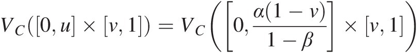 (3.41)
VC([0, u] × [v, 1]) = C(u, 1) − C(u, v) − C(0, 1) + C(0, v) = u − C(u, v)VC0u×v1=Cu1−Cuv−C01+C0v=u−Cuv(3.42)
VC0α1−v1−β×v1=Cα1−v1−β1−Cα1−v1−βv−C01+C0v=α1−v1−β−Cα1−v1−βvEquating Equation (3.42) to Equation (3.43), we get the following: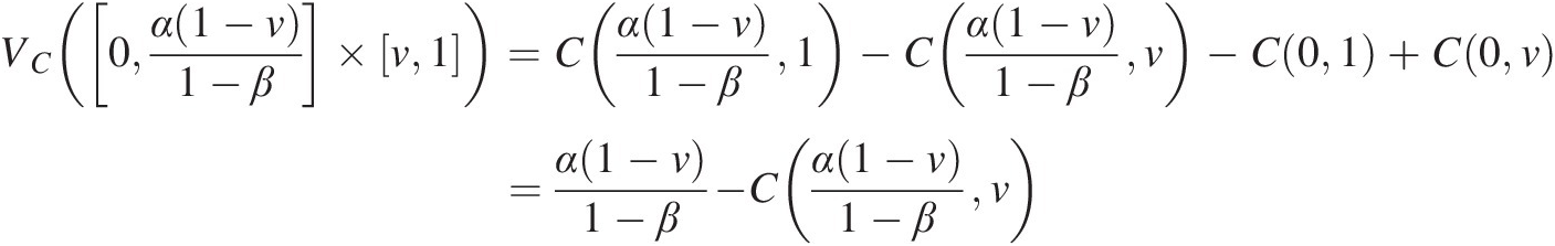 (3.43)
Cuv=u−α1−v1−βIn order to determine the copula function in this region, we can also look at the rectangle α1−v1−βu×v1.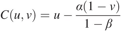 (3.44a)
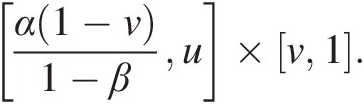 This rectangle is not intercepting any support line segment, thus we know the C-volume is zero, as follows:
VCα1−v1−βu×v1=Cu1−Cuv−Cα1−v1−β1+Cα1−v1−βv=0⇒Cuv=u−α1−v1−β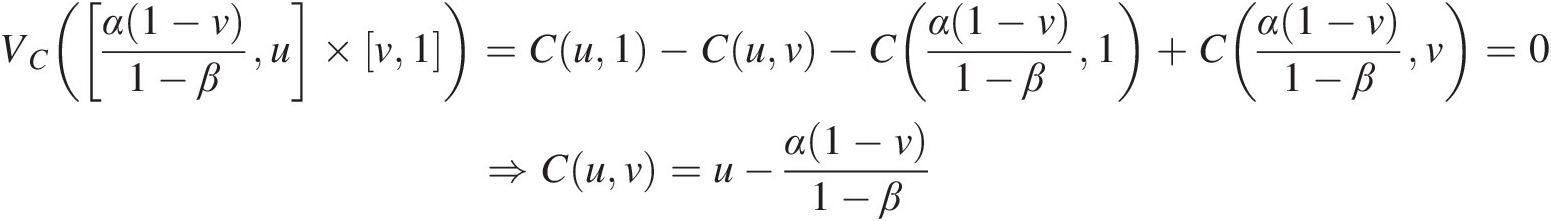 (3.44b)
2. Similarly, If (u,v) falls into the region bounded by the lower triangular region with vertices (α,β), (1, 0), and (1, 1), as shown in Figure 3.2(c), then we can use the same approach to find the following:
Cuv=v−β1−α1−u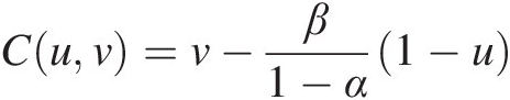 (3.45)
3. If (u,v) is not falling into the two triangles bounded by the support segment, then we immediately know that the C-volume is zero and C(u, v)Cuv can be found as follows:
VC([0, u] × [0, v]) = C(u, v) − C(0, v) − C(u, 0) − C(0, 0) = 0 ⇒ C(u, v) = 0VC0u×0v=Cuv−C0v−Cu0−C00=0⇒Cuv=0(3.46)


Note the following for the limiting cases:
1. If α = β = 0α=β=0, the support line segment is the main diagonal on I2. Nelsen (2006) proved that in this case, C(u, v)Cuv is the Fréchet–Hoeffding upper bound, i.e., C(u, v) = M(u, v) = min (u, v)Cuv=Muv=minuv.
2. If β = 1 − αβ=1−α, Equation (3.44a) and Equation (3.45) reduce to the following:
Cuv=u−β1−α1−v=u+v−1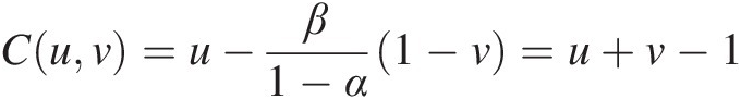 (3.47a)
and
Cuv=v−α1−β1−u=u+v−1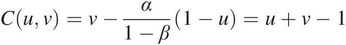 (3.47b)
Equation (3.47) represents the Fréchet–Hoeffding lower bound, i.e.,
C(u, v) = W(u, v) = max (u + v − 1, 0)Cuv=Wuv=maxu+v−10.(3.47)


Figure 3.2 Schematic of singular copulas with prescribed support.
Example 3.11 Copulas with prescribed horizontal or vertical support.
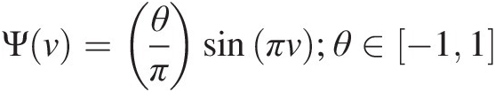
Show for each of the following choices of the ΨΨ function, the function C given as
is a copula:
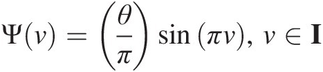
a. Ψv=θπsinπv;θ∈−11
b. Ψ(v) = θ[ζ(v) + ζ(1 − v)], θ ∈ [−1, 1]; ζΨv=θζv+ζ1−v,θ∈−11;ζ is the piecewise linear function with the graph connecting [0, 0] to (1/4, 1/4) to (1/2, 0) to (1, 0).

Solution: According to Nelsen (2006), if Equation (3.48) is a copula, it is a copula with quadratic sections in u.
a. Ψv=θπsinπv,θ∈−11
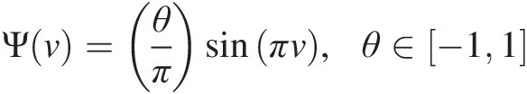

Corollary 3.2.5 (from Nelsen, 2006) can be applied to prove that the C function with the ΨΨ function so defined is a copula. Corollary 3.2.5 states the necessary and sufficient conditions for the C function to be a copula:
1. Ψ(v)Ψv is absolutely continuous on I.
2. |Ψ‘(v)| ≤ 1Ψ’v≤1 almost everywhere on I.
3. |Ψ(v)| ≤ min (v, 1 − v)Ψv≤minv1−v.
Based on corollary 3.2.5, we conclude the following:
1. It is easy to see that Ψ(v)Ψv is absolutely continuous on I with sine function being an absolutely continuous function.
2. It is seen that for θ ∈ [−1, 1], |θ/π| < 1θ∈−11,θ/π<1, so we have the following: ∣Ψ’v∣=∣θπcosπv∣<1
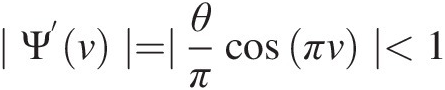 .
.
3. For Ψv=θπsinπv,v∈I
 , we have the following:
0≤πv≤π,sinπv≤πv⇒Ψv=θπsinπv≤θππv=θv≤v (3.49)
Similarly,
sinπv=sinπ−πv=sinπ1−v≤π1−v⇒Ψv=θπsinπ1−v≤θ1−v≤1−v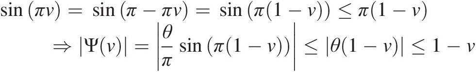 (3.50)
From Equations (3.49) and (3.50), we have |Ψ(v)| ≤ min (v, 1 − v)Ψv≤minv1−v for v ∈ Iv∈I.


Now, all the conditions are satisfied and function C with Ψ(v)Ψv defined in a. is a copula.
b. Ψ(v) = θ[ζ(v) + ζ(1 − v)], θ ∈ [−1, 1]Ψv=θζv+ζ1−v,θ∈−11; ζζ is the piecewise linear function with the graph connecting {[0, 0] to (1/4, 1/4)} to {(1/2, 0) to (1, 0)}.
Theorem 3.2.4 in Nelsen (2006) can be applied to prove that function C is a copula. Theorem 3.2.4 states the necessary and sufficient conditions for C to be a copula as follows:
1. Ψ(0) = Ψ(1) = 0Ψ0=Ψ1=0
2. Ψ(v)Ψv satisfies the Lipschitz condition: |Ψ(v2) − Ψ(v1)| ≤ |v2 − v1|; v1, v2 ∈ IΨv2−Ψv1≤v2−v1;v1,v2∈I
3. C is absolutely continuous.
The schematic plot for the piecewise linear function is given in Figure 3.3(a).

Figure 3.3 Plots of functions ζ(v)ζv and Ψ(v)Ψv.
The Ψ(v)Ψv function can be written as follows:
 (3.51)
1. For θ ∈ [−1, 1]θ∈−11, we have the following:
Ψ(0) = 0; Ψ(1) = θ(1 − 1) = 0Ψ0=0;Ψ1=θ1−1=0
2. Prove the Lipschitz condition with v1 ≤ v2v1≤v2 and θ ∈ [−1, 1]θ∈−11.
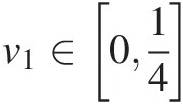
i. If v1∈014
 , we have the following:
|Ψ(v2) − Ψ(v2)|Ψv2−Ψv2
=θv2−v1≤v2−v1;v2∈014θ12−v2−θv1=θ12−v1+v2<θv2−v1≤v2−v1;v2∈1434θv2−1−θv1<θv2−v1−1<v2−v1;v2∈341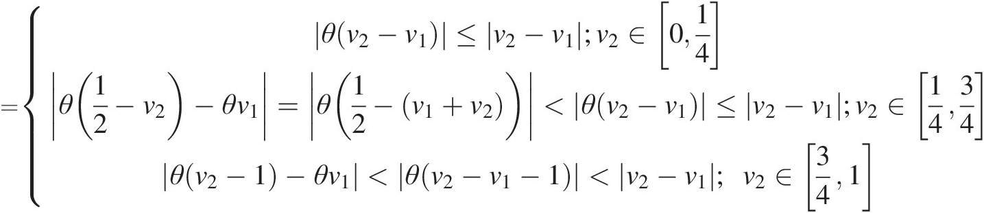 (3.52)
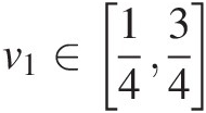
ii. If v1∈1434
 , we have the following:
Ψv2−Ψv1=θ12−v2−θ12−v1=θv2−v1≤v2−v1;v2∈1434θv2−1−θ12−v1=∣θ(v2+v1−32∣≤θv2−34≤θv2−v1≤v2−v1;v2∈341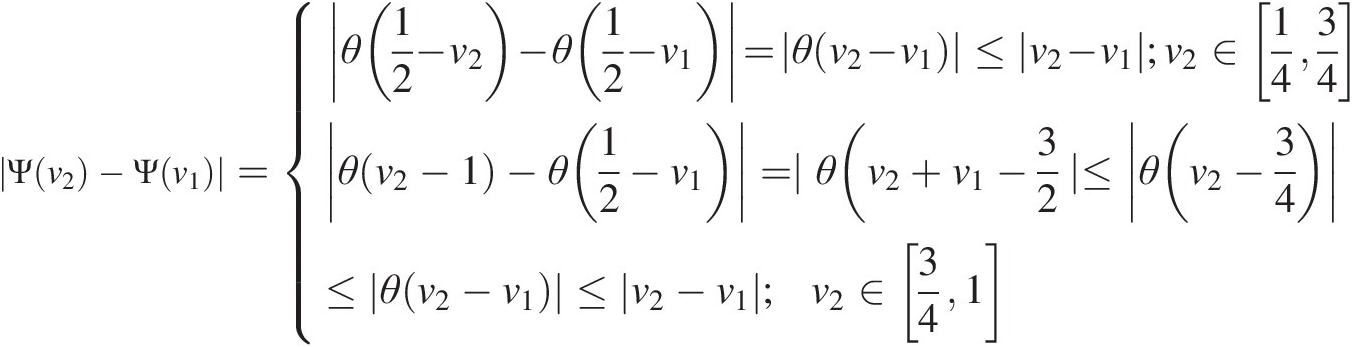 (3.53)
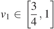
iii. Similarly, it can be easily shown that the Lipschitz condition is also satisfied for v1∈341
 .
.
3. Following Nelsen (2006), to prove the absolute continuity of C follows the absolute continuity of Ψ(v)Ψv with the second condition. Figure 3.3(b) plots the Ψ(v)Ψv function with θ = 0.8θ=0.8; as an example, it is shown that there is no discontinuity in domain I:
Ψ’v=θ,v∈014−θ,v∈1434θ,v∈341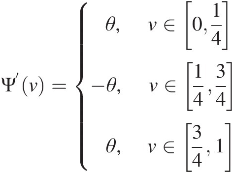 (3.54)
with θ ∈ [−1, 1]θ∈−11, we have proved that |Ψ‘(v)| ≤ 1Ψ’v≤1 in domain I.


Now all the conditions are satisfied and the C function with the Ψ(v)Ψv function defined in (b) is a copula.
It is worth noting that the copula defined as Equation (3.48) is a copula with quadratic sections in u. The reader can refer to Nelsen (2006) for more complete details of the geometric method and other types of geometric support to construct copulas.
3.2.3 Algebraic Method
Copulas may be constructed using the algebraic relationship between joint distribution and univariate distributions of random variables X1 and X2, which is called the algebraic method. Nelsen (2006) introduced this approach by constructing the Plackett and Ali–Mikhail–Haq copula through an “odd” ratio in which the Plackett copula is constructed by measuring the dependence of two-by-two contingency tables, and Ali–Mikhail–Haq copula is constructed by using the survival odds ratio. In order to discuss the method, the Ali–Mikhail–Haq copula construction example presented in Nelsen (2006) is used here.
The survival odds ratio for a univariate random variable X with X ~F(x) can be expressed as follows:
 (3.55)
Similarly, the survival odds ratio for bivariate random variables X1 and X2 with joint distribution F (x1, x2) and marginals F1(x1), F2(x2)F1x1,F2x2 can be expressed as follows:
 (3.56)
Example 3.12 The Ali–Mikhail–Haq copula.
The Ali–Mikhail–Haq copula (Ali et al., 1978) can be expressed as follows:
 (3.57)
Construct the copula by using the algebraic method.
Solution: Ali et al. (1978) proposed that Ali–Mikhail–Haq copula belongs to the bivariate logistic distribution family with the standard bivariate logistic distribution and standard logistic marginals.
The standard bivariate logistic distribution can be given as follows:
The standard logistic marginal can be given as follows:
The survival ratio of Equation (3.58a) is
 (3.59)
From Equation (3.59), it is seen that the survival ratio of the standard bivariate logistic distribution can be rewritten as follows:
 (3.60a)
Substituting Equation (3.58b) into Equation (3.60a), we have the following:
 (3.60b)
In Ali et al. (1978), the Ali–Mikhail–Haq copula was considered a bivariate distribution satisfying the survival ratio as follows:
 (3.61)
It is concluded from Equation (3.61) that θ = 1 implies that the joint distribution F(x, y) of random variables X1X1 and X2X2 follows the standard biviariate logistic distribution; and θ = 0 implies that X and Y are independent with the proof given in example 3.19 in Nelsen (2006).
Applying Sklar’s theorem to Equation (3.59) and letting
Equation (3.61) can be rewritten as follows:
 (3.62)
With simple algebra, we have
 (3.63)
where θ is the parameter of the Ali–Mikhail–Haq copula.
3.3 Families of Copula
There are a multitude of copulas. Generally speaking, copulas may be grouped into the Archimedean copulas, meta-elliptical copulas, and copulas with prescribed geometric support (e.g., copulas with quadratic or cubic sections). According to their exchangeable properties, copulas may also be classified as symmetric copulas and asymmetric copulas. For example, one-parameter Archimedean copulas are symmetric copulas, and periodic copulas (Alfonsi and Brigo, 2005) and mixed copulas (Hu, 2006) are asymmetric copulas. Here we will only discuss the general concepts of each copula family. The copula functions pertaining to a given copula family will be discussed in detail in subsequent chapters.
3.3.1 Archimedean Copulas
Archimedean copulas are widely applied in finance, water resources engineering, and hydrology due to their simple form, dependence structure, and other “nice” properties. Chapters 4 and 5 discuss the symmetric and asymmetric Archimedean copulas.
3.3.2 Plackette Copula
The Plackette copula has been applied in recent years. It will be discussed in Chapter 6.
3.3.3 Meta-elliptical Copulas
Meta-elliptical copulas are a flexible tool for modeling multivariate data in hydrology. They will be further discussed in Chapter 7.
3.3.4 Entropic Copula
Similar to the entropy-based univariate probability distributions, the entropy theory (e.g., Shannon entropy) may be applied to derive entropic copulas with the use of constraints in regard to the total probability theory, properties of marginals (i.e., EUi=1i+1 ), and the dependence measure (e.g., Spearman rank-based correlation coefficient). The entropic copula will be further discussed in Chapter 8.
3.3.5 Mixed Copulas
Parametric copulas place restrictions on the dependence parameter. When data are heterogeneous, it is desirable to have additional flexibility to model the dependence structure (Trivedi and Zimmer, 2007). A mixture model, proposed by Hu (2006), is able to measure dependence structures that do not belong to the aforementioned copula families. By choosing component copulas in the mixture, a model can be constructed that is simple and flexible enough to generate most dependence patterns and provide such a flexibility in practical data. This also facilitates the separation of the degree of dependence and the structure of dependence. These concepts are respectively embodied in two different groups of parameters: the association parameters and the weight parameters (Hu, 2006). For example, the given bivariate data may be modeled as a finite mixture with three bivariate copulas CI(u, v), CII(u1, u2), CIII(u1, u2)CIuv,CIIu1u2,CIIIu1u2; the mixture model is defined as follows:
where Cmix(u, v; θ1, θ2, θ3, w1, w2)Cmixuvθ1θ2θ3w1w2w3 denotes the mixed copula; CI(u, v; θ1), CII(u, v; θ2), CIII(u, v; θ3)CIuvθ1,CIIuvθ2,CIIIuvθ3 are the three bivariate copulas, each with θ1, θ2, θ3θ1,θ2,θ3 as the corresponding copula parameters; and w1, w2, w3w1,w2,w3 may be interpreted as weights for each copula such that 0<wj<1;j=1,2,3,∑j=13wj=1,0<wj<1 .
.
3.3.6 Empirical Copula
Sometimes, we analyze data with an unknown underlying distribution. The empirical data distribution can be transformed into what is called an “empirical copula” by warping such that the marginal distributions become uniform. Let x1 and x2 be two samples each of size n. The empirical copula frequency function can often be computed for any pair (x1, x2)x1x2 by
 (3.65)
where {(x1i, x2j) : 0 ≤ i, j ≤ n}x1ix2j:0≤ij≤n represent, respectively, the ith- and jth-order statistic of x1 and x2.
Example 3.13 Using the peak discharge (Q: m3/s) and flood volume (V: m3) given in Table 3.1, calculate the empirical copula with the use of Equation (3.65).
Table 3.1. Peak discharge and flood volume data (from Yue, 2001).
| Pair | Year | V (m3) | Q (cms) | Pair | Year | V (m3) | Q (cms) |
|---|---|---|---|---|---|---|---|
| 1 | 1942 | 8,704 | 371 | 28 | 1969 | 11,272 | 416 |
| 2 | 1943 | 6,907 | 245 | 29 | 1970 | 8,640 | 246 |
| 3 | 1944 | 4,189 | 189 | 30 | 1971 | 6,989 | 248 |
| 4 | 1945 | 8,637 | 229 | 31 | 1972 | 9,352 | 297 |
| 5 | 1946 | 8,409 | 240 | 32 | 1973 | 12,825 | 371 |
| 6 | 1947 | 13,602 | 331 | 33 | 1974 | 13,608 | 442 |
| 7 | 1948 | 8,788 | 206 | 34 | 1975 | 8,949 | 260 |
| 8 | 1949 | 5,002 | 157 | 35 | 1976 | 12,577 | 236 |
| 9 | 1950 | 5,167 | 184 | 36 | 1977 | 11,437 | 334 |
| 10 | 1951 | 10,128 | 275 | 37 | 1978 | 9,266 | 310 |
| 11 | 1952 | 12,035 | 286 | 38 | 1979 | 14,559 | 383 |
| 12 | 1953 | 10,828 | 230 | 39 | 1980 | 5,057 | 151 |
| 13 | 1954 | 8,923 | 233 | 40 | 1981 | 9,645 | 197 |
| 14 | 1955 | 11,401 | 351 | 41 | 1982 | 7,241 | 283 |
| 15 | 1956 | 6,620 | 156 | 42 | 1983 | 13,543 | 390 |
| 16 | 1957 | 3,826 | 168 | 43 | 1984 | 15,003 | 405 |
| 17 | 1958 | 8,192 | 343 | 44 | 1985 | 6,460 | 176 |
| 18 | 1959 | 6,414 | 214 | 45 | 1986 | 7,502 | 181 |
| 19 | 1960 | 8,900 | 303 | 46 | 1987 | 5,650 | 233 |
| 20 | 1961 | 9,406 | 300 | 47 | 1988 | 7,350 | 187 |
| 21 | 1962 | 7,235 | 143 | 48 | 1989 | 9,506 | 216 |
| 22 | 1963 | 8,177 | 232 | 49 | 1990 | 6,728 | 196 |
| 23 | 1964 | 7,684 | 182 | 50 | 1991 | 13,315 | 424 |
| 24 | 1965 | 3,306 | 121 | 51 | 1992 | 8,041 | 255 |
| 25 | 1966 | 8,026 | 186 | 52 | 1993 | 10,174 | 257 |
| 26 | 1967 | 4,892 | 173 | 53 | 1994 | 14,769 | 232 |
| 27 | 1968 | 8,692 | 292 | 54 | 1995 | 8,711 | 286 |
Solution: To determine the empirical copula, we will first need to rank the flood volume and peak discharge variables in the increasing order. Then we can use Equation (3.65) to compute the empirical copula. Here we will use C1n1n as an illustration example. For the flood data in Table 3.1, Table 3.2 lists the order statistics of flood volume and peak discharge individually.
Table 3.2. Order statistics of flood volume and peak discharge.
| Order | V (m3 day/s) | Q (cms) | Order | V (m3 day/s) | Q (cms) |
|---|---|---|---|---|---|
| 1 | 3,306 | 121 | 28 | 8,704 | 245 |
| 2 | 3,826 | 143 | 29 | 8,711 | 246 |
| 3 | 4,189 | 151 | 30 | 8,788 | 248 |
| 4 | 4,892 | 156 | 31 | 8,900 | 255 |
| 5 | 5,002 | 157 | 32 | 8,923 | 257 |
| 6 | 5,057 | 168 | 33 | 8,949 | 260 |
| 7 | 5,167 | 173 | 34 | 9,266 | 275 |
| 8 | 5,650 | 176 | 35 | 9,352 | 283 |
| 9 | 6,414 | 181 | 36 | 9,406 | 286 |
| 10 | 6,460 | 182 | 37 | 9,506 | 286 |
| 11 | 6,620 | 184 | 38 | 9,645 | 292 |
| 12 | 6,728 | 186 | 39 | 10,128 | 297 |
| 13 | 6,907 | 187 | 40 | 10,174 | 300 |
| 14 | 6,989 | 189 | 41 | 10,828 | 303 |
| 15 | 7,235 | 196 | 42 | 11,272 | 310 |
| 16 | 7,241 | 197 | 43 | 11,401 | 331 |
| 17 | 7,350 | 206 | 44 | 11,437 | 334 |
| 18 | 7,502 | 214 | 45 | 12,035 | 343 |
| 19 | 7,684 | 216 | 46 | 12,577 | 351 |
| 20 | 8,026 | 229 | 47 | 12,825 | 371 |
| 21 | 8,041 | 230 | 48 | 13,315 | 371 |
| 22 | 8,177 | 232 | 49 | 13,543 | 383 |
| 23 | 8,192 | 232 | 50 | 13,602 | 390 |
| 24 | 8,409 | 233 | 51 | 13,608 | 405 |
| 25 | 8,637 | 233 | 52 | 14,559 | 416 |
| 26 | 8,640 | 236 | 53 | 14,769 | 424 |
| 27 | 8,692 | 240 | 54 | 15,003 | 442 |
To apply the empirical copula, using x(1) = 3360, y(1) = 121x1=3360,y1=121 as an example, we have C1n1n represent #(xi ≤ x(1) & yi ≤ y(1), i = 1, 2, …, 54)/54#(xi≤x1&yi≤y1i=12…54)/54. Looking up Table 3.1, we find that there is only one pair, i.e., pair 24 (3360, 121), that satisfies the condition x(1) = 3360x1=3360 and y(1) = 121y1=121. Thus, we have C154154=154
 . With this in mind, we can easily compute the empirical copula for the rest of the values, as shown in Figure 3.4.

3.4 Dependence Measure
There are several measures of dependence or association among variables. Five popular measures are Pearson’s classical correlation coefficient r, Spearman’s ρρ, Kendall’s ττ, chi-plots, and K-plots. These dependence measures were originally developed in the field of nonparametric statistics. Pearson’s classical correlation coefficient is also called the linear correlation coefficient or simply correlation coefficient (i.e., sensitive to linear dependence). Spearman’s ρρ and Kendall’s ττ are rank-based correlation coefficients based on the concordance and discordance of the dataset. Compared to the classic Pearson correlation coefficient, the rank-based correlation coefficients are more robust. Here, we first use the sample data to illustrate the dependence measurement, then we will show another example using the hydrological data.
3.4.1 Pearson’s Classical Correlation Coefficient r and Spearman’s ρρ
Consider a continuous bivariate random variable (X1, X2X1,X2) with marginal distributions F1(x1)F1x1 and F2(x2)F2x2. Spearman’s ρρ is given by
where r denotes Pearson’s linear correlation coefficient.
In other words, rank-based Spearman’s ρρ represents Pearson’s linear correlation coefficient between variables u = F1(x1), v = F2(x2)u=F1x1,v=F2x2. Because u and v are both uniform [0, 1] random variables with mean 1/2 and variance 1/12, Spearman’s ρρ in Equation (3.66) can be rewritten as
 (3.67)
In terms of copulas, substituting u = F1(x1), v = F2(x2)u=F1x1,v=F2x2 in Equation (3.67), Spearman’s ρρ is then
 (3.68)
After some simple algebra, Equation (3.68) can be rewritten (Schweizer and Wolff, 1981) as follows:
 (3.69)
The pairwise empirical Spearman ρnρn can be expressed as follows:
 (3.70)
where nn is the sample size; RiRi is the rank of xixi among x1, …, xnx1,…,xn; and SiSi is the rank of yiyi among y1, …, yny1,…,yn; R¯=S¯=1n∑i=1n;Ri=1n∑i=1n;Si=n+12.
Example 3.14 Table 3.3 lists six learning datasets {(xi, yi) : i = 1, …, 6}xiyi:i=1…6. Calculate the rank-based correlation coefficient Spearman’s ρnρn.
Table 3.3. Learning datasets.
| i | 1 | 2 | 3 | 4 | 5 | 6 |
|---|---|---|---|---|---|---|
| xixi | 7.476 | 11.375 | 3.595 | 9.635 | 10.731 | 13.942 |
| yiyi | 8.441 | 8.952 | 0.700 | 10.645 | 3.665 | 9.793 |
Solution: The rank of the dataset is computed as in Table 3.4 and Figure 3.5.
Table 3.4. Rank of the learning datasets.
| i | 1 | 2 | 3 | 4 | 5 | 6 |
|---|---|---|---|---|---|---|
| xixi | 7.476 | 11.375 | 3.595 | 9.635 | 10.731 | 13.942 |
| RiRi | 2 | 5 | 1 | 3 | 4 | 6 |
| yiyi | 8.441 | 8.952 | 0.700 | 10.645 | 3.665 | 9.793 |
| SiSi | 3 | 4 | 1 | 6 | 2 | 5 |

Figure 3.5 Scatter plot of ranked pairs (Ri, Si), chi-plot, and K-plot to detect the dependence for the dataset in Table 3.3. (a) Scatter plot of (Ri, Si); (b) chi-plot with control limit of P = 0.9, 0.95; and (c) K-plot with independent and perfectly positively dependent curves.
Using Equation (3.70), we have the following:


3.4.2 Kendall’s τ
Consider two independent and identically distributed continuous bivariate random variables, (X1, X2)X1X2 and X1∗X2∗ , where F1(x1)F1x1 denotes the marginal distribution for X1X1 and X1∗
 , and the marginal distribution F2(x2)F2x2 for X2X2 and X2∗.
 Then, Kendall’s τ is given by
 (3.71)
In Equation (3.71), the first term measures concordance, and the second term measures discordance. Therefore, Kendall’s correlation coefficient τ can be rewritten as
 (3.72)
Now empirical Kendall’s τ (τn) from bivariate observations can be written as
 (3.73)
where nn is the number of observations. sign⋅=1;∃x1i−x1jx2i−x2j>00;∃x1i−x1jx2i−x2j=0−1;∃x1i−x1jx2i−x2j≤0.
In terms of the copula function, Kendall’s τ can be expressed from Equation (3.71) as follows:
 (3.74)
From Equation (3.74), we also know the following:
 (3.75)
Let u = F1(x1), v = F2(x2), C(u, v) = P(x1, x2)u=F1x1,v=F2x2,Cuv=Px1x2 PX1<X1∗X2<X2∗=PX1≤X1∗X2≤X2∗ for continuous random variables. Substituting Equation (3.75) into Equation (3.74), we have the following:
 (3.76)
Example 3.15 Calculate Kendall’s τnτn for the data of Table 3.3.
Solution: To calculate sample Kendall’s τnτn, we will use Equation (3.73). To illustrate the calculation procedure, we will use the first pair (x1 = 15.237, y1 = 19.2x1=15.237,y1=19.2) as an example shown in Table 3.5.
Table 3.5. Sample results of computing Kendall’s tau.
| Variable | (x1 − x2)(y1 − y2)x1−x2y1−y2 | (x1 − x3)(y1 − y3)x1−x3y1−y3 | (x1 − x4)(y1 − y4)x1−x4y1−y4 | (x1 − x5)(y1 − y5)x1−x5y1−y5 | (x1 − x6)(y1 − y6)x1−x6y1−y6 |
|---|---|---|---|---|---|
| Result | > 0 | > 0 | < 0 | > 0 | > 0 |
| Sign (●) | 1 | 1 | 1 | –1 | 1 |
| Sum | 3 |
Similarly, we can compute the sum for the remaining pairs as follows:
Pair (x2, y2)x2y2 compared to {(xi, yi) : i = 3, …, 6}xiyi:i=3…6, sum = 2;
Pair (x3, y3)x3y3 compared to {(xi, yi) : i = 4, …, 6}xiyi:i=4…6, sum = 3;
Pair (x4, y4)x4y4 compared to {(xi, yi) : i = 5, 6}xiyi:i=56, sum = –2;
Pair (x5, y5)x5y5 compared to (x6, y6)x6y6, sum = –1;
Finally, using Equation (3.73), we have the following:

3.4.3 Chi-plot
The chi-plot is based on the chi-square statistic for independence in a two-way table. For bivariate random variables (X1, X2)X1X2, let Hi=∑j=1n1x1j≤x1ix2j≤x2ij≠in−1,Fi=∑j=1n1x1j≤x1ij≠in−1, and Gi=∑j=1n1x2j≤x2ij≠in−1
 ; the chi-plot can be determined using pairs (λi, χi)λiχi following Fisher and Switzer (2001) and Genest and Favre (2007) as follows:
 (3.77)
 (3.78)
where F˜i=Fi−12;G˜i=Gi−12 .
.
To avoid outliers, Fisher and Switzer (2001) recommended that what should be plotted are only the pairs for which
 (3.79)
To detect how far apart the bivariate random variable is from independence, Fisher and Switzer (2001) also suggested the “control limit” estimated as follows:
 (3.80)
where CL stands for the “control limit” that may also be considered as the confidence bound for independence; n is the sample size; and cp is the critical value to guarantee that the 100p% of the pair (λi, χi)λiχi falls into the control limit, i.e., for p = 0.9, 0.95, 0.99p=0.9,0.95,0.99, cp = 1.54, 1.78, 2.18cp=1.54,1.78,2.18, respectively.
Example 3.16 Calculate the chi-plot for the data of Table 3.3.
Solution: Using Equations (3.71) and (3.72), we have the pairs (λi, χi),λiχi, as shown in Table 3.6 and Figure 3.5.
Table 3.6. Coordinates of points, displayed on the chi-plot, for the data of Table 3.3.
| ii | 1 | 2 | 3 | 4 | 5 | 6 |
|---|---|---|---|---|---|---|
| HiHi | 0.2 | 0.6 | 0 | 0.4 | 0.2 | 0.8 |
| FiFi | 0.2 | 0.8 | 0 | 0.4 | 0.6 | 1 |
| GiGi | 0.4 | 0.6 | 0 | 1 | 0.2 | 0.8 |
F˜i | –0.3 | 0.3 | –0.5 | –0.1 | 0.1 | 0.5 |
G˜i | –0.1 | 0.1 | –0.5 | 0.5 | –0.3 | 0.3 |
| χiχi | 0.61 | 0.61 | — | — | 0.41 | — |
| λiλi | 0.36 | 0.36 | 1 | –1 | –0.36 | 1 |
From Table 3.6, it is seen that only three pairs satisfy the condition, and the control limit for p = 0.9, 0.95, 0.99p=0.9,0.95,0.99 will be CL = ± 0.63, ± 0.73, ± 0.89,CL=±0.63,±0.73,±0.89, respectively.
3.4.4 K-plot
The K-plot was first proposed by Genest and Boies (2003). It is another rank-based graphical tool for detecting dependence. The K-plot consists in plotting pairs (Wi : n, H(i)), i = 1, …, nWi:nHi,i=1,…,n, where H(1) < … < H(n)H1<…<Hn are the order statistics associated with quantities H1 < … < HnH1<…<Hn, i.e.,
Hi=∑j=1n1x1j≤x1ix2j≤x2ij≠in−1 .
.
Based on the null hypothesis, i.e., H0: U and V (or equivalently X and Y) are independent, Genest and Favre (2007) stated that Wi : nWi:n is the expected value of the ith statistic from a random sample of size n from the random variable W = C(U, V) = H(X, Y)W=CUV=HXY as follows:
 (3.81)
where
K0w=PUV<w=∫01PU≤wvdv=∫0w1dv+∫w1wvdv=w−wlnw
and

Similar to the chi-plot, the K-plot is also capable of detecting how far apart dependence is from independence. We already know the following relations in terms of copula function, i.e., Π = uv; M = min (u, v), W = max (u + v − 1, 0)Π=uv;M=minuv,W=maxu+v−10 for the independent, perfectly positively dependent, and perfectly negatively dependent bivariate random variables, respectively. Graphically, on the K-plot, (i) the (Wi : n, H(i))Wi:nHi pairs follow a straight line x2 = x1x2=x1, i.e., H(i) = Wi : nHi=Wi:n if X and Y are independent; (ii) the (Wi : n, H(i))Wi:nHi pairs follow the K0(w)K0w curve, if X and Y are perfectly positively dependent; and (iii) the (Wi : n, H(i))Wi:nHi pairs fall onto the x1-axis, i.e., W(i : n)Wi:n, if X and Y are perfectly negatively dependent.
Example 3.17 Calculate the K-plot for the data of Table 3.3.
Solution: Let f(x) = xk0(w){K0(x)}i − 1{1 − K0(x)}n − 1; n = 6fx=xk0wK0xi−11−K0xn−1;n=6. We can obtain Wi : nWi:n with the numerical integration. The results are given in Table 3.7 and Figure 3.5.
Table 3.7. Coordinates of points displayed on the K-plot for the data of Table 3.3.
| ii | 1 | 2 | 3 | 4 | 5 | 6 |
|---|---|---|---|---|---|---|
| Wi : nWi:n | 0.04 | 0.09 | 0.16 | 0.26 | 0.38 | 0.57 |
| H(i)Hi | 0 | 0.2 | 0.2 | 0.4 | 0.6 | 0.8 |
| K0K0 | 0.16 | 0.31 | 0.46 | 0.60 | 0.75 | 0.89 |
Example 3.18 Using the peak discharge and flood volume data given in Table 3.1, (1) calculate sample Spearman’s ρn and Kendall’s τn; and (2) graph the chi-plot and K-plot.
Solution: Table 3.8 lists the rank of flood volume (VV) and peak discharge (QQ). The computation procedure is exactly the same as that in Examples 3.14–3.17.
1. Calculate the sample Spearman’s ρn and Kendall’s τn:
Using Equation (3.70) and the same procedure as in Example 3.14, we can easily compute sample ρn = 0.7577ρn=0.7577 using Table 3.8 with sample size of 54, as follows:

Using Equation (3.73) and the same procedure as in Example 3.15, we can compute sample Kendall’s τn as τn = 0.5695τn=0.5695.
Table 3.8. Rank ([RV, RQ]RVRQ) of the bivariate flood variables.
| RVRV | V(m3) | RQRQ | Q(cms) | RVRV | V(m3) | RQRQ | Q(cms) |
|---|---|---|---|---|---|---|---|
| 28 | 8,704 | 47.5 | 371 | 42 | 11,272 | 52 | 416 |
| 13 | 6,907 | 28 | 245 | 26 | 8,640 | 29 | 246 |
| 3 | 4,189 | 14 | 189 | 14 | 6,989 | 30 | 248 |
| 25 | 8,637 | 20 | 229 | 35 | 9,352 | 39 | 297 |
| 24 | 8,409 | 27 | 240 | 47 | 12,825 | 47.5 | 371 |
| 50 | 13,602 | 43 | 331 | 51 | 13,608 | 54 | 442 |
| 30 | 8,788 | 17 | 206 | 33 | 8,949 | 33 | 260 |
| 5 | 5,002 | 5 | 157 | 46 | 12,577 | 26 | 236 |
| 7 | 5,167 | 11 | 184 | 44 | 11,437 | 44 | 334 |
| 39 | 10,128 | 34 | 275 | 34 | 9,266 | 42 | 310 |
| 45 | 12,035 | 36.5 | 286 | 52 | 14,559 | 49 | 383 |
| 41 | 10,828 | 21 | 230 | 6 | 5,057 | 3 | 151 |
| 32 | 8,923 | 24.5 | 233 | 38 | 9,645 | 16 | 197 |
| 43 | 1,1401 | 46 | 351 | 16 | 7,241 | 35 | 283 |
| 11 | 6,620 | 4 | 156 | 49 | 13,543 | 50 | 390 |
| 2 | 3,826 | 6 | 168 | 54 | 15,003 | 51 | 405 |
| 23 | 8,192 | 45 | 343 | 10 | 6,460 | 8 | 176 |
| 9 | 6,414 | 18 | 214 | 18 | 7,502 | 9 | 181 |
| 31 | 8,900 | 41 | 303 | 8 | 5,650 | 24.5 | 233 |
| 36 | 9,406 | 40 | 300 | 17 | 7,350 | 13 | 187 |
| 15 | 7,235 | 2 | 143 | 37 | 9,506 | 19 | 216 |
| 22 | 8,177 | 22.5 | 232 | 12 | 6,728 | 15 | 196 |
| 19 | 7,684 | 10 | 182 | 48 | 13,315 | 53 | 424 |
| 1 | 3,306 | 1 | 121 | 21 | 8,041 | 31 | 255 |
| 20 | 8,026 | 12 | 186 | 40 | 10,174 | 32 | 257 |
| 4 | 4,892 | 7 | 173 | 53 | 14,769 | 22.5 | 232 |
| 27 | 8,692 | 38 | 292 | 29 | 8,711 | 36.5 | 286 |
Given the double summation for the computation of sample Kendall’s tau, here we will show the first intersummation (i.e., i = 1, j = 2:54), or in other words, comparing (V, Q) = (8704, 371)VQ=8704371 to the rest of pairs:
Taking the summation, we have sumi = 1 = 14sumi=1=14.
Proceeding with i = 2i=2 till i = 53i=53, we have the following:
and we have the following:
τn=25454−114+22+29+…−1=0.5695
2. Graph the chi-plot and K-plot:
Chi-plot: Using Equations (3.77)–(3.80) with the same procedure as given in Example 3.16, let Fi = FVFi=FV and Gi = FQGi=FQ; Fi, GiFi,Gi may be directly computed using Fi=RV53,Gi=RQ53 from the rank listed in Table 3.8. HiHi is similar to the empirical copula, which is computed and listed in Table 3.8. Now we can compute and graph the chi-plot for correlated peak discharge and flood volume variables.
K-plot: Using Equation (3.81) with the same procedure as given in Example 3.17, we may compute and graph the K-plot for correlated peak discharge and flood volume variables. The K-plot involves integration; we can simply use the integral function in MATLAB to obtain results. Figure 3.6 graphs the scatter and chi- and K-plots for correlated peak discharge and flood volume variables.

Figure 3.6 Scatter plot of observed data, chi-plot, and K-plot for the hydrological dataset.
(a) Scatter plot of observed data; (b) chi-plot with P = 0.9, 0.95; and (c) K-plot with independent and perfectly positive dependent curves.
From this example, we see that from calculated sample Spearman’s ρn and Kendall’s τn, the peak discharge and flood volume are positively dependent. The chi-plot and K-plot also graphically indicate a positive dependence structure between peak discharge and flood volume.
3.5 Dependence Properties
The dependence between random variables is important for multivariate analysis. Joe (1997), Nelsen (2006), among others, studied the dependence properties of copulas in detail. Here we present the important dependence properties, including positive quadrant and orthant dependence, stochastically increasing positive dependence, right-tail increasing and left-tail decreasing dependence, positive function dependence, and tail dependence.
3.5.1 Positive Quadrant and Orthant Dependence
The positive quadrant dependence (PQD) may be expressed as follows:
or
in which X1, X2 are the random variables with margins F1(x1)F1x1 and F2(x2),F2x2, respectively.
Similarly, X1, X2 are negative quadrant dependent (NQD), if the following relationship is satisfied:
or
Considering multivariate variables (dimension ≥ 3), the positive upper/lower orthant dependent (PUOD/PLOD) may take place (Joe, 1997). Let X be a random vector with dimension n (n ≥ 3) with multivariate distribution function H, then PUOD/PLOD states the following:
i. X or H is PUOD if for vector a, a ∈ ℜna∈ℜn such that
PXi>aii=1…n≥∏i=1nPXi>ai (3.84)
ii. X or H is PLOD if for vector a, a ∈ ℜna∈ℜn such that
PXi≤aii=1…n≥∏i=1nPXi≤ai (3.85)


Similarly, X or H is NUOD if for vector a, a ∈ ℜna∈ℜn such that
 (3.86)
and X or H is NLOD if for vector a, a ∈ ℜna∈ℜn such that
 (3.87)
It is seen from Equations (3.84) and (3.85) that multivariate random variables X1, …, Xn are more likely having large values simultaneously, compared to the independence assumption. Similarly, Equations (3.86) and (3.87) show that multivariate random variables X1, …, Xn are more likely having small values simultaneously, compared to the independence assumption.
Example 3.19 Explain that the following Gumbel–Houggard copula holds the positive quadrant dependence property.
 (3.88)
Solution: From Equation (3.88), with θ ≥ 1θ≥1, we have the Kendall correlation coefficient τ ∈ [0, 1]τ∈01. With the robust Kendall correlation, it is guaranteed that the random variables are positively dependent. From the theorem of Fréchet–Hoeffding bounds, the product copula (i.e., Π = uvΠ=uv) represents independence (i.e., τ = 0τ=0) and M = min (u, v)M=minuv represents the perfectly correlated random variables (i.e., τ = 1τ=1) with the relation of Π ≤ MΠ≤M. Then we have the following: Π < C(u, v) < MΠ<Cuv<M for the positively correlated random variables with 0 < τ < 10<τ<1:
The preceding relation aligns with Equation (3.82b) and holds the positive quadrant property. To illustrate this property graphically, we will use θ = 2.5θ=2.5 as an example:

Figure 3.7 plots the comparison of Equation (3.88) and product copula with different pairs of (u, v)uv. Figure 3.7 graphically shows that the JCDF computed using Equation (3.89) with θ = 2.5θ=2.5 is greater than that computed from the product copula (i.e., fulfilling Equation (3.82b)).

3.5.2 Stochastic Increasing Positive Dependence
Bivariate Stochastic Positive Dependence
Let there be random variables X1, X2 with the joint probability distribution, F(x1, x2)Fx1x2, and marginal F1(x1), F2(x2)F1x1,F2x2. Then, X1 is stochastically increasing (SI) in X2, or, in other words, the conditional probability distribution F(X1|X2) is stochastically increasing, if the following relationship exists:
is a nondecreasing function of x1x1 for all x2x2.
Similarly, we say X1 is stochastically decreasing (SD) in X2 if P(X1>x| X2 = x2)PX1>xX2=x2 is a nonincreasing function of x1x1 for all x2x2.
Multivariate Stochastic Positive Dependence
As introduced by Joe (1997), a random vector X, X = (X1, X2, …, Xn) is stochastically positive dependent if {Xi: i ≠ j} conditional on Xj = x is increasing stochastically, as x increases for all j = 1, …, n. The random vector X is conditional increasing in sequence in X1, …, Xi–1 for i = 2, …, n, if P(Xi>xi| Xj = xj, j = 1, 2, …, i − 1)PXi>xiXj=xjj=12…i−1 is increasing in x1, …, xi–1 for all xi.
Example 3.20 Rework Example 3.19 to evaluate the stochastic dependence property for the copula given in Equation (3.88) with θ = 2.5θ=2.5.
Solution: We first derive the conditional probability distribution as follows:
 (3.89)
Taking the partial derivative of Equation (3.89), we have the following:
 (3.90a)
 (3.90b)
Again let v = 0.2, 0.5, 0.7v=0.2,0.5,0.7. Figure 3.8 plots Equation (3.90). Figure 3.8a plots the conditional copula (i.e., conditional cumulative distribution function) with different v. Figure 3.8b plots the exceedance conditional copula (i.e., the exceedance conditional distribution) with different v. Figure 3.8b clearly shows that the exceedance conditional copula is nondecreasing for any given u with increasing v, i.e., C(u| V = 0.2) ≤ C(u| V = 0.5) ≤ C(u| V = 0.7)CuV=0.2≤CuV=0.5≤CuV=0.7. This indicates the stochastic increasing (SI) property of the copula function given in Equation (3.88).

Figure 3.8 Comparison of the conditional copula (i.e., P(X ≤ x| Y = y)PX≤xY=y) and the exceedance conditional copula (i.e., P(X>x| Y = y)PX>xY=y).
3.5.3 Tail Dependence
Nelsen (2006) introduced the tail dependence as follows.
Population Version of Tail Dependence
Let X1 and X2 be two random variables. Then,
a. X2 is left tail decreasing (LTD) in X1, i.e., LTD (X2|X1), if P(X2 ≤ x2| X1 ≤ x1)PX2≤x2X1≤x1 is a nonincreasing function of x1x1 for all x2x2. Similarly, if P(X1 ≤ x1| X2 ≤ x2)PX1≤x1X2≤x2 is a nonincreasing function of x2x2 for all x1x1, then there exists LTD (X1|X2).
b. X2 is left tail increasing (LTI) in X1, i.e., LTI (X2|X1), if P(X2 ≤ x2| X1 ≤ x1)PX2≤x2X1≤x1 is a nondecreasing function of x1x1 for all x2x2. Similarly, if P(X1 ≤ x1| X2 ≤ x2)PX1≤x1X2≤x2 is a nondecreasing function of x2x2 for all x1x1, then there exists LTI (X1|X2).
c. X2 is right tail increasing (RTI) in X1, i.e., RTI (X2|X1), if P(X2>x2| X1>x1)PX2>x2X1>x1 is a nondecreasing function of x1x1 for all x2x2. Similarly, if P(X1>x1| X2>x2)PX1>x1X2>x2 is a nondecreasing function of x2x2 for all x1x1, then there exists RTI (X1|X2).
d. X2 is right tail decreasing (RTD) in X1, i.e., RTD (X2|X1), if P(X2>x2| X1>x1)PX2>x2X1>x1 is a nonincreasing function of x1x1 for all x2x2. Similarly, if P(X1>x1| X2>x2)PX1>x1X2>x2 is a nonincreasing function of x2x2 for all x1x1, then there exists RTD (X1|X2).
Copula Version of Tail Dependence
The copula version of tail dependence is given as Theorem 5.2.5 in Nelsen (2006).
Let X1, X2 be continuous random variables with margins u = F1(x1); v = F2(x2)u=F1x1;v=F2x2 and the joint distribution represented by copula C. Then, the theorem says the following:
a. There exists LTD (X1|X2) if and only if for any v in I = [0,1], such that C(u, v)/vCuv/v is nonincreasing in u. Similarly, LTD (X2|X1) exists if and only if for any u in I = [0,1], such that C(u, v)/uCuv/u is nonincreasing in v.
b. There exists RTI (X1|X2) if and only if for any v in I = [0,1], such that [1 − u − v + C(u, v)]/(1 − v)1−u−v+Cuv/1−v is nondecreasing in v, or equivalently, if [u − C(u, v)]/(1 − v)u−Cuv/1−v is nonincreasing in v. Similarly, RTI (X2|X1) exists if and only if for any u in i = [0,1], such that [1 − u − v + C(u, v)]/(1 − u)1−u−v+Cuv/1−u is nondecreasing in u, or equivalently, if [v − C(u, v)]/(1 − u)v−Cuv/1−u is nonincreasing in u.
Example 3.21 Rework Example 3.20 to evaluate that the tail dependence of the copula function given in Equation (3.88) with parameter θ = 2.5θ=2.5 holds the RTI property.
Solution: To show the copula function (3.88) holds the RTI property, we need to show that P(X1>x1| X2>x2)PX1>x1X2>x2 is a nondecreasing function of x2x2 for all x1x1 or equivalently to show that [u − C(u, v)]/(1 − v)u−Cuv/1−v is nonincreasing in v. Similar to previous two examples, we will again use v = 0.2, 0.5, 0.7v=0.2,0.5,0.7 as an illustrative example. Figure 3.9 plots the exceedance joint distribution and corresponding [u − C(u, v)]/(1 − v)u−Cuv/1−v for u = 0 : 0.01 : 0.99u=0:0.01:0.99. Figure 3.9(b) shows that given V>vV>v, the conditional copula C(U>u| V>v)CU>uV>v is a nonincreasing function on v. In other words, C(U>u| V>v)CU>uV>v decreases for V>vV>v with the increase of v. Thus, the copula function given in Equation (3.88) holds the RTI property. Using three pairs of (u,v), (0.3,0.2), (0.3,0.5), and (0.3, 0.7), for an illustrative example, we have the following:

Theoretically, we can prove the RTI property by taking the first-order derivative with respect to v and have the following:
 (3.91)
To show the copula function (i.e., Equation (3.90)) holds the RTI property, we need to show that Equation (3.91) is equal to or less than 0 in what follows:
 (3.92)
Taking the first-order derivative of Equation (3.88) with respect to v, we have the following:
 (3.93)
In Equation (3.93), we have the following inequalities:
 (3.94)
Substituting Equation (3.94) back into Equation (3.93), Equation (3.92) may be rewritten as follows:
 (3.95)
Equation (3.95) proves that the Equation (3.93) is equal to or less than 0, i.e., [u − C(u, v)]/(1 − v)u−Cuv/1−v is a nonincreasing function of v. Hence, the copula function in Equation (3.88) holds the RTI property.

Figure 3.9 Graphical evaluation of tail dependence for copula function (Equation (3.90)).
3.5.4 Likelihood Ratio Dependence
The likelihood ratio dependence was discussed as Theorem 5.2.18 in Nelsen (2006). This theorem says that if there are two continuous random variables X1 and X2 whose joint density function is f(x1, x2)fx1x2, then X1 and X2 are positively likelihood ratio dependent if the following inequality is satisfied:
 (3.96)
for all x1,x2,x1′,x2′ in R¯
in R¯ such that x1≤x1′,x2≤x2′
 . This is also called the total positivity of power 2 (TP2) (Joe, 1997).
The preceding discussion introduces the dependence structure and properties of the copulas that are most important for multivariate analysis in later chapters.
3.6 Copula Parameter Estimation
For a d-dimensional random sample (X1, X2, …, Xd)X1X2…Xd with marginal distribution F1(X1), …, Fd(Xd)F1X1,…,FdXd, let f(X1, …, Xd)fX1…Xd be the joint density function of the d-dimensional random variables and F(X1, …, Xd)FX1…Xd be the corresponding joint distribution. Here we discuss some general methods used to estimate copula parameters.
3.6.1 Exact Maximum Likelihood Estimation Method
The exact maximum likelihood estimation method is also called the one-stage method or full maximum likelihood (full ML). The full ML method estimates the parameters of marginal distributions and copula function simultaneously. Let Θ = (α1, …, αd, θ)Θ=α1…αdθ be the parameters that need to be estimated in which αi, i = 1, …, d,αi,i=1,…,d, is the parameter for marginal variable XiXi and θθ is the copula parameter. Based on the relation between copula density and joint density function of d-dimensional variables, i.e., fX1…XdΘ=cU1…Udθ∏i=1dfiXiαi , the log-likelihood function is given as follows:
 (3.97)
The log-likelihood function can be maximized numerically by solving for ΘΘ, i.e.,

as follows:
 (3.98)
Equation (3.98) shows that with increasing scale of the problem, the algorithm can be too burdensome computationally.
3.6.2 Inference Function for Marginal Method
In the inference function for margins (IFM) method, a two-stage method, i.e., the parameters of marginal distribution and copula function are estimated separately. First, parameter αiαi of the marginal distribution F̂iXiαi is estimated; and then the fitted marginal distribution is passed into the copula function to estimate its parameter θθ.
1. The log-likelihood function of each of the marginal distributions is given as
logLαi=∑j=1nlnfxijαi;i=1,2,…d (3.99)
αiαi is estimated by α̂i=argmaxlogLαi
 , i.e.,
∂logLαi∂αi=0 (3.100)
2. With the fitted marginal distributions, the log-likelihood function for the copula can be given as
logLα̂1…α̂dθ=∑i=1nlnF1x1iα̂1…Fdxdiα̂dθ (3.101)


Maximizing Equation (3.101) over θθ,
θ̂IFM=argmaxlogLθ
which is estimated by setting the following:
 (3.102)
Comparing the IFM method with the full ML method, the IFM method is computationally more efficient than the full ML method. However, if the marginal distribution is misidentified, the accuracy of the copula (or joint distribution) estimated will be undermined.
The semiparametric approach provides the ability to avoid the misidentification of marginal distributions and is discussed in the following section.
3.6.3 Semiparametric Method
The semiparametric method is more flexible. In this method, copula parameters are estimated with the maximum likelihood estimation method, using nonparametric empirical distribution functions rather than the fitted parametric marginals. Using the commonly applied Weibull plotting position formula, the empirical probability is written as follows:
 (3.103)
Replacing the fitted marginal distribution in Equation (3.101) with the results obtained from Equation (3.103), the copula parameters can be estimated by maximizing the following pseudo-log-likelihood function:
 (3.104)
For a set of copula candidates, the copula function reaching the largest log-likelihood is usually considered as the best-fitted copula to represent the multivariate distribution function for given multivariate continuous random variables.
In what follows, we will give one synthetic example to illustrate how to apply the preceding three methods to estimate the copula parameters.
Example 3.22 Using the correlated random variables.
This example uses the correlated random variables listed in Table 3.9 with the assumption of random variables X and Y following the gamma and Gumbel distributions, respectively, and the joint distribution following the Gumbel–Houggard copula as follows:

Estimate the parameters using the previously discussed full ML, IFM, and semiparametric methods.
Table 3.9. Synthetic random variables.
| No. | X | Y |
|---|---|---|
| 1 | 2.3284 | 16.2698 |
| 2 | 0.8867 | 8.6807 |
| 3 | 1.4106 | 11.2295 |
| 4 | 1.9654 | 12.1751 |
| 5 | 1.0221 | 7.5978 |
| 6 | 1.2089 | 8.8760 |
| 7 | 0.6915 | 9.0297 |
| 8 | 1.5375 | 10.2731 |
| 9 | 1.9472 | 13.4256 |
| 10 | 1.0080 | 8.9696 |
| 11 | 2.2308 | 10.2306 |
| 12 | 0.7600 | 7.4901 |
| 13 | 1.7782 | 11.1462 |
| 14 | 3.6810 | 15.2615 |
| 15 | 2.4564 | 13.1492 |
| 16 | 4.1957 | 19.5030 |
| 17 | 2.5038 | 12.4057 |
| 18 | 3.6670 | 16.4510 |
| 19 | 0.4646 | 5.9375 |
| 20 | 1.1004 | 10.1990 |
| 21 | 0.4608 | 10.1966 |
| 22 | 2.0799 | 11.5089 |
| 23 | 0.9049 | 9.2902 |
| 24 | 0.5785 | 7.4861 |
| 25 | 1.1199 | 9.1667 |
| 26 | 1.9836 | 13.0043 |
| 27 | 0.8940 | 8.6892 |
| 28 | 3.6308 | 17.6573 |
| 29 | 1.4556 | 10.5674 |
| 30 | 1.8813 | 9.4640 |
Solution: Before we proceed to estimate the parameters, we first give the density function for the Gumbel–Houggard copula as follows:

Full ML method: The gamma and Gumbel density functions can be given as follows:
Gamma: fXxαxβx=βxαxxαx−1Γαxe−βxx ;
;
Gumbel: fYyμyβy=1βyexp−y−μyβy+exp−y−μyβy
Now, the joint density function, i.e., f(x, y)fxy can be expressed as follows:
The log-likelihood function of f(x, y)fxy can be expressed as follows:

Now, by maximizing the preceding log-likelihood function with the use of Equations (3.97) and (3.98), we can estimate all five parameters simultaneously. One may also use the optimization toolbox in MATLAB to estimate the parameters by minimizing the negative log-likelihood function. Here we use the optimization toolbox in MATLAB to estimate the parameters. The estimated parameters and corresponding log-likelihood value are listed in Table 3.10.
Table 3.10. Estimated parameters using full ML, IFM, and semiparametric methods.
| Method | Univariate | Copula | ||
|---|---|---|---|---|
| X~gamma(αx, βx)X~gammaαxβx | Y~gumbel(μy, βy)Y~gumbelμyβy | GH (θ)GHθ | LL | |
| Full ML | (3.0691, 0.5674) | (9.7235, 2.5083) | 3.5236 | –87.4934 |
| IFM | (3.0782, 0.5613) | (9.7271, 2.4681) | 3.4760 | 25.8129 |
| Semiparametric | – | – | 3.5570 | 23.6911 |
IFM method: The IFM method estimates the parameters of marginals and copula function separately.
First, we need to estimate the parameters for the marginal distributions using the ML method as follows:
Second, we use the fitted probability distribution to compute the cumulative probability listed in Table 3.11.
Table 3.11. Estimated cumulative distributions using fitted and empirical probability distributions.
| X | Gamma | Empirical | Y | Gumbel | Empirical |
|---|---|---|---|---|---|
| 2.3284 | 0.7695 | 0.7742 | 16.2698 | 0.9318 | 0.8710 |
| 0.8867 | 0.1967 | 0.1935 | 8.6807 | 0.2170 | 0.1613 |
| 1.4106 | 0.4404 | 0.4516 | 11.2295 | 0.5804 | 0.6129 |
| 1.9654 | 0.6628 | 0.6452 | 12.1751 | 0.6901 | 0.6774 |
| 1.0221 | 0.2583 | 0.3226 | 7.5978 | 0.0935 | 0.1290 |
| 1.2089 | 0.3464 | 0.4194 | 8.8760 | 0.2437 | 0.2258 |
| 0.6915 | 0.1166 | 0.1290 | 9.0297 | 0.2654 | 0.2903 |
| 1.5375 | 0.4969 | 0.5161 | 10.2731 | 0.4486 | 0.5161 |
| 1.9472 | 0.6567 | 0.6129 | 13.4256 | 0.7997 | 0.8065 |
| 1.0080 | 0.2517 | 0.2903 | 8.9696 | 0.2568 | 0.2581 |
| 2.2308 | 0.7439 | 0.7419 | 10.2306 | 0.4424 | 0.4839 |
| 0.7600 | 0.1431 | 0.1613 | 7.4901 | 0.0841 | 0.0968 |
| 1.7782 | 0.5954 | 0.5484 | 11.1462 | 0.5697 | 0.5806 |
| 3.6810 | 0.9550 | 0.9355 | 15.2615 | 0.8992 | 0.8387 |
| 2.4564 | 0.7999 | 0.8065 | 13.1492 | 0.7788 | 0.7742 |
| 4.1957 | 0.9773 | 0.9677 | 19.5030 | 0.9811 | 0.9677 |
| 2.5038 | 0.8103 | 0.8387 | 12.4057 | 0.7133 | 0.7097 |
| 3.6670 | 0.9542 | 0.9032 | 16.4510 | 0.9365 | 0.9032 |
| 0.4646 | 0.0458 | 0.0645 | 5.9375 | 0.0096 | 0.0323 |
| 1.1004 | 0.2950 | 0.3548 | 10.1990 | 0.4378 | 0.4516 |
| 0.4608 | 0.0448 | 0.0323 | 10.1966 | 0.4375 | 0.4194 |
| 2.0799 | 0.6999 | 0.7097 | 11.5089 | 0.6152 | 0.6452 |
| 0.9049 | 0.2047 | 0.2581 | 9.2902 | 0.3031 | 0.3548 |
| 0.5785 | 0.0777 | 0.0968 | 7.4861 | 0.0838 | 0.0645 |
| 1.1199 | 0.3042 | 0.3871 | 9.1667 | 0.2851 | 0.3226 |
| 1.9836 | 0.6690 | 0.6774 | 13.0043 | 0.7672 | 0.7419 |
| 0.8940 | 0.1999 | 0.2258 | 8.6892 | 0.2181 | 0.1935 |
| 3.6308 | 0.9520 | 0.8710 | 17.6573 | 0.9606 | 0.9355 |
| 1.4556 | 0.4607 | 0.4839 | 10.5674 | 0.4909 | 0.5484 |
| 1.8813 | 0.6336 | 0.5806 | 9.4640 | 0.3287 | 0.3871 |
Third, use the computed cumulative probability from the fitted probability distribution to estimate the copula parameter by maximizing the log-likelihood function of copula density function or minimizing its negative log-likelihood function. Again using the optimization toolbox in MATLAB, the fitted copula parameters and their log-likelihood value are listed in Table 3.10.
Semiparametric method: The semiparametric method estimates the parameter of copula function using the empirical marginal distributions, which is free of identification of marginal distributions.
First, we use the Weibull probability plotting-position formula to compute the empirical probabilities, which are listed in Table 3.11.
Second, we estimate the copula parameter using the computed empirical probabilities. Here we again use the optimization toolbox in MATLAB to estimate the parameters. The estimated parameter and the corresponding log-likelihood value are listed in Table 3.11.
Table 3.10 shows that the parameters of marginal distributions, estimated using the full ML method, are very close to those estimated separately by the IFM method. The copula parameter values estimated using all three methods are also very close to each other.
3.7 Copula Simulation
A common simulator for copula is the cumulative probability integral (CPI) Rosenblatt transformation. Let X = (X1, X2, …, Xd)X=X1X2…Xd be a d-dimensional, absolutely continuous random variable, H(x1, x2, …, xd)Hx1x2…xd the joint distribution function, and FXi(xi) = P(Xi ≤ xi), i = 1, 2, …, d, the univariate marginalsFXixi=PXi≤xi,i=1,2,…,d,the univariate marginals. In what follows, we introduce how to simulate copula samples using the CPI Rosenblatt transformation (Rosenblatt, 1952). The Rosenblatt transformation can be written as follows:
…
 (3.107)
Let U(0, 1) denote the uniform distribution on [0,1]. The following procedure generates a d-dimensional random variate (u1, …, ud)u1…ud from copula C(u1, …, ud) = Cd(u1, …, ud)Cu1…ud=Cdu1…ud:
1. Simulate independent random variates v1, …, vdv1,…,vd from U(0, 1)U01 and set u1 = v1u1=v1.
2. Simulate random variate u2u2 from v2 = C2(u2| u1)v2=C2u2u1 by solving u2=C2∣1−1v2u1
 .
.
…
3. Simulate random variate udud from vd = Cd(ud| u1, …, ud − 1)vd=Cdudu1…ud−1 by solving
ud=Cd∣1,…,d−1−1vdu1…ud−1.


The Clayton copula is as follows:

Solution: First, generate two independent random variates (v1, v2)v1v2 from U(0, 1)U01, and set u1 = v1u1=v1. Then,

Solving the equation v2 = C(u2| u1)v2=Cu2u1 for u2u2 yields

Using a synthetic example with generated independently uniformly distributed random variate (0.6036, 0.4028) with the copula parameter θ = 0.5 (Clayton copula), set the following:
Then we can compute the following:

3.8 Goodness-of-Fit Tests for Copulas
Besides choosing the copula function that reaches the largest log-likelihood (or minimum negative log-likelihood, Akaike information criterion [AIC], Bayesian information criterion [BIC]) from possible copula functions tested, the goodness-of-fit test further ensures the appropriateness of the selected copula functions. Currently, there exist seven formal goodness-of-fit tests for copulas: (1) two tests based on the empirical copula with test statistics: Sn, TnSn,Tn; (2) two tests based on Kendall’s transform with test statistics: SnK,TnK ; and (3) three tests based on Rosenblatt’s transform with test statistics: An,SnB,SnC
 . Sn,SnK,SnB
 , and SnC
 , which are calculated based on Cramér–von Mises statistics; and Tn,TnK
 , which are calculated based on the Kolmogorov–Smirnov statistics. According to Genest et al. (2007), the preference ranking for these goodness-of-fit tests is SnB≻Sn≻SnC≻Tn≻An≻TnK
 . In this section, we present procedures on how to calculate the goodness-of-fit statistics for bivariate random variables following Genest et al. (2007). All the preceding test statistics can be extended to higher dimensions using the same procedures. In what follows, we will discuss the goodness-of-fit procedures. The examples will be provided in the later chapters.
3.8.1 Goodness-of-Fit Test Based on Empirical Copula: Sn, TnSn,Tn
The goodness-of-fit statistics SnSn and TnTn are based on the empirical copula. Similar to the univariate Cramér–von Mises and Kolmogorov–Smirnov goodness-of-fit tests, the test based on the empirical copula is to compare the distance between the empirical copula (Cn) and the parametric copula (Cθ) fitted to the pseudo-observations under the null hypothesis H0 (the given parametric copula function cannot be rejected). The goodness-of-fit test statistics, i.e., Cramér–von Mises test statistic (Sn)Sn) and Kolmogorov–Smirnov test statistic (Tn)Tn) for an empirical copula can be written as follows:
where
 (3.108c)
In Equations (3.108a)–(3.108c), Cn(u)Cnu is the empirical copula calculated from Equation (3.65) or using the following formula (Genest et al., 2007):
 (3.109)
This is the fitted copula function and n is the sample size.
If there is an analytical expression for Cθ̂,Sn,Tn , then that may be calculated directly using Equations(3.108a)–(3.108c). Otherwise, Monte Carlo simulation is applied for m > n as follows:
1. Generate a bivariate random sample U1∗,U2∗
 from Cθ̂
 .
.
2. Approximate Cθ̂
 by
by
Bm∗=1m∑i=1m1Ui∗≤u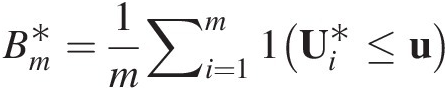 (3.110)
3. Approximate SnSn by
Sn=∑i=1nCnUi−Bm∗Ui2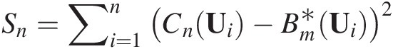 (3.111a)
Tn=supu∈012nCnUi−Bm∗Ui (3.111b)


With the fitted copula function, the P-value of the test statistic is approximated using parametric bootstrap simulation repeated for some large integer N times as follows:
1. Generate a bivariate sample X1∗,X2∗
 from the copula function Cθ̂
 and compute the associated rank vectors: R1∗,R2∗
 .
.
2. Compute Ui=Rin+1
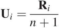 and let
Cn∗=1n∑i=1nUi∗≤u (3.111c)
3. Estimate the copula parameter from Ui∗
 for the tested copula function.
4. Calculate the test statistics either directly using Equations (3.108a)–(3.108c) or approximated using Equations (3.111a) and (3.111b).


Finally, the P-value of the test statistic is approximated as follows:
 (3.112)
3.8.2 Goodness-of-Fit Test Based on Kendall’s Transform: SnK,TnK

The goodness-of-fit test SnK and TnK
 are based on the probability integral transform, i.e., Kendall’s transform with mapping as follows:
According to Genest et al. (2007), let K represent the univariate distribution function of V. K may be estimated nonparametrically using the empirical distribution function of the rescaled version of pseudo-observations V1 = Cn(u1), …, Vn = Cn(un)V1=Cnu1,…,Vn=Cnun with the use of the following equation:
 (3.114)
The null hypothesis (H0) is that u = [u1, u2]u=u1u2 may be modeled by the copula function CθCθ or equivalently, the Kendall transform of Cθ(u)Cθu follows the distribution KθKθ. Measuring the distance between KnKn(the empirical Kendall transform) and the parametric estimation KθnKθn of K into the goodness-of-fit test may be performed through Cramér–von Mises (SnK) and Kolmogorov–Smirnov (TnK
 ) statistics as follows:
 (3.115a)
 (3.115b)
where
 (3.115c)
In Equations (3.115a)–(3.115c), if there is an analytical expression for KθnKθn, the test statistics can be directly computed. Otherwise, Monte Carlo simulation with m ≥ nm≥n will be needed to approximate KθnKθn as follows:
1. Generate a random sample u1∗,u2∗,…,um∗
 from the fitted copula function CθnCθn.
2. Approximate KθnKθn using the following:
Bm∗=1m∑i=1m1Vi∗≤t,t∈01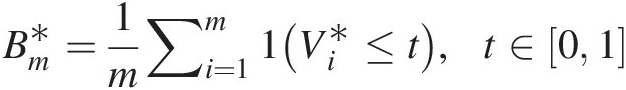 (3.116)
where
Vi∗=1m∑j=1m1uj∗≤ui∗,i=1,2,…,n
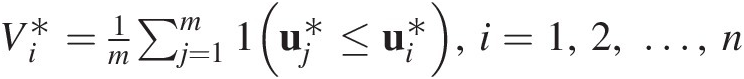
3. Approximate SnK
 and TnK
 using the following equations:
SnK=nm∑i=1mKnVi∗−Bm∗Vi∗2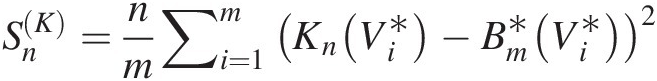 (3.117a)
TnK=supV∈01nKnV∗−Bm∗V∗ (3.117b)


For the fitted copula function, the P-value of the goodness-of-fit test is approximated using a similar parametric bootstrap simulation repeated for some large number N times as follows:
1. Generate random sample X1,k∗,…,Xn,k∗
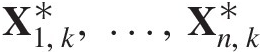 from the fitted copula function CθnCθn and compute their associated rank R1,k∗,…,Rn,k∗
 .
.
2. Compute
Vi,k∗=1n∑j=1n1Xj,k∗≤Xi,k∗,i=1,…,n (3.118a)
Kn,k∗t=1n∑i=1n1Vi,k∗≤t,t∈01 (3.118b)
3. Assign U1,k∗=R1,k∗n+1,…,Un,k∗=Rn,k∗n+1
 and reestimate the parameters for the copula function.
4. If there is an analytical expression for KθKθ, then calculate Sn,kK∗
 and Tn,kK∗
 using Equations (3.115a)–(3.115c). Otherwise, Kθn,k∗
 needs to be approximated using the procedure discussed earlier in this section to estimate Sn,kK∗
 and Tn,kK∗
 .
.


Finally, the P-value of the test statistic can be written as follows:
 (3.119)
It is worth noting that this goodness-of-fit test is most sensitive to the copula functions with analytical Kendall’s distribution, i.e., Archimedean copulas.
3.8.3 Goodness-of-Fit Test Based on Rosenblatt’s Transform: An,SnB,SnC

Based on Rosenblatt’s transform discussed through Equations (3.105)–(3.107), Rosenblatt’s transform for the bivariate random variables with a joint distribution represented by a copula function Cθ(u1, u2); u1 = FX1(x1); u2 = FX2(x2)Cθu1u2;u1=FX1x1;u2=FX2x2 can be expressed as follows:
The null hypothesis (H0) of the goodness-of-fit test based on Rosenblatt’s transform is that u = [u1, u2]~Cθu=u1,u2~Cθ, i.e., Z1, Z2Z1,Z2, is a bivariate independent copula, as follows:
In the preceding three test statistics, theAnAn-test statistic is also called the Anderson–Darling test statistic such that the chi-square distribution is assumed as the limiting distribution. Compared to AnAn, SnB and SnC
 do not assume the chi-square distribution as the limiting distribution; the latter two tests are also called the goodness-of-fit tests based on an improved Rosenblatt’s transform (Genest et al., 2007). Cramér–von Mises statistic is considered for both SnB
 and SnC
 . These two tests are further discussed in what follows.
Under the null hypothesis, let the empirical distribution be written as follows:
 (3.122)
From Equation (3.121), it is known that Z1 and Z2 should be “close” to independently uniformly distributed random variables, i.e., C⊥C⊥. Then the distance between Dn(u)Dnu and C⊥C⊥ is used to construct the goodness-of-fit test SnB and SnC
 , as follows:
 (3.123)
where Zik ∨ Zjk = max (Zik, Zjk)Zik∨Zjk=maxZikZjk.
 (3.124)
For the fitted copula function, the P-value of the statistic is also determined, based on the parametric bootstrap simulation repeated for some large integer N times as follows:
1. Generate a random sample {X1, X2}X1X2 with the same sample size as the original dataset, from the estimated copula function Cθ̂
 and compute the rank vectors: R1∗R2∗
 .
.
2. Compute the intermediate variables as follows:
U1∗=R1∗n+1,U2∗=R2∗n+1 (3.125)
3. Reestimate the copula parameter θ̂∗
 using U1∗
 and U2∗
 with the same copula function, and compute Z1∗
 , Z2∗
, Z2∗ using Equation (3.120).
4. Compute Sn,kB∗
 and Sn,kC∗
 using Equations (3.123) and (3.124), respectively.
5. After repeating steps 1 through 4 N times, the P-value can be given as follows:
Pvalue=1N∑k=1N1Sn,kB∗>SnBorPvlaue=1N∑k=1NSn,kC∗>SnC (3.126)


3.9 Procedure for Multivariate Frequency Analysis
The procedure for multivariate frequency analysis is sketched in Figure 3.10.

Figure 3.10 Procedure for multivariate frequency analysis.
3.10 Joint/Conditional Distributions and Corresponding Return Periods through Copulas
In multivariate frequency analysis, the following probability distributions are useful for hydrologic and environmental applications. In this section, applications are discussed for bivariate and trivariate cases using the following:
3.10.1 Calculation of Joint Probability for Bivariate and Trivariate Cases
Joint Probability for Bivariate Events
Using bivariate variables X1 and X2 as an example, the joint probabilities can be expressed as follows:
 (3.127)
Joint Probability for Trivariate Events
For trivariate random variables X1, X2, and X3, common formulas of trivariate probability distributions can be given as follows:
 (3.130)
 (3.131)
 (3.132)
 (3.133)
 (3.134)
 (3.135)
 (3.136)
3.10.2 Return Periods through Copulas
A return period, also known as a recurrence interval, is an estimate of the interarrival time between events, such as earthquakes, floods, or river discharge flows of a certain intensity or size. It is a statistical measurement denoting the average recurrence interval over an extended period of time and is usually required for risk analysis (i.e., whether a project should be allowed to go forward in a zone with a certain risk) and infrastructure engineering design purposes (i.e., designing structures so that they are capable of withstanding an event of a certain return period).
In hydrology and water resources engineering, the return period (also called recurrence interval) T is the average time interval between occurrences of the event X ≥ xX≥x for unviariate case. That is, T is defined as the average recurrence interval for events X ≥ xX≥x (i.e., Equation (2.81) in Chapter 2), as follows:
 (3.137)
Equation (3.137) also shows the relation among return period T, nonexceedance probability FX(x)FXx, and exceedance probability F¯Xx . Hence, we also have
 (3.138)
Using the same concept for the univariate case, the return period can be estimated for multivariate cases. Here we present the bivariate and trivariate cases. Examples will be given in the later chapters.
Bivariate Case: Joint Return Period Using Copulas
“AND” case: X1>x1 and X2>x2X1>x1andX2>x2
The joint return period of the “AND” case can be expressed by substituting Equation (3.127) into Equation (3.137) as follows:
 (3.139)
The joint return period of the “OR” case is simply expressed as follows:
 (3.140)
Equation (3.140) indicates the combination of the following:
Case: X1>x1 and X2 ≤ x2 (or X1 ≤ x1and X2>x2)X1>x1andX2≤x2orX1≤x1andX2>x2:
For illustrative purposes, we use X1>x1X1>x1 and X2 ≤ x2X2≤x2 as an example. From Equation (3.128),
 (3.142)
Similarly, the return period of X1>x1X1>x1 and X2 ≤ x2X2≤x2 is as follows:
 (3.143)
Bivariate Case: Conditional Return Period Using Copulas
The copula can be used to determine the conditional distribution functions and conditional return periods under different conditions.
Case: X2>x2 ∣ X1 = x1X2>x2∣X1=x1 (or X1>x1 ∣ X2 = x2X1>x1∣X2=x2):
Using X2>x2 ∣ X1 = x1X2>x2∣X1=x1 as an example, the conditional probability of X2 ≤ x2 ∣ X1 = x1X2≤x2∣X1=x1 can be written as follows:
 (3.144)
Given that P(X2 ≤ x2| X1 = x1) + P(X2>x2| X1 = x1) = 1PX2≤x2X1=x1+PX2>x2X1=x1=1, we have the following:
 (3.145)
Then, the corresponding conditional return period is as follows:
 (3.146a)
Similarly, the conditional return period of X1>x1 ∣ X2 = x2X1>x1∣X2=x2 is as follows:
 (3.146b)
Case: X2>x2 ∣ X1 ≤ x1X2>x2∣X1≤x1 (or X1>x1 ∣ X2 ≤ x2X1>x1∣X2≤x2)
Again, using X2>x2 ∣ X1 ≤ x1X2>x2∣X1≤x1, the conditional distribution of X2 ≤ x2 ∣ X1 ≤ x1X2≤x2∣X1≤x1 is expressed using copula as follows:
 (3.147)
Then we have the following:
 (3.148a)
Likewise, we have the following:
 (3.148b)
Trivariate Case: Joint Return Period Using Copulas
Similar to the bivariate case, the joint return periods for the trivariate case are also discussed as the “AND” case:
X1>x1 ∩ X2>x2 ∩ X3>x3X1>x1∩X2>x2∩X3>x3
X1>x1 ∪ X2>x2 ∪ X3>x3X1>x1∪X2>x2∪X3>x3.
“AND” case: X1>x1 ∩ X2>x2 ∩ X3>x3X1>x1∩X2>x2∩X3>x3
In this case, all three values of X1, X2, and X3 are exceeded. Applying Equation (3.136), the return period TAND(x1, x2, x3)TANDx1x2x3 can be given as follows:
 (3.149)
“OR” case: X1>x1 ∪ X2>x2 ∪ X3>x3X1>x1∪X2>x2∪X3>x3
In this case, at least one value of X1, X2, and X3 is exceeded and the joint return period TOR(x1, x2, x3)TORx1x2x3 can be given as follows:
 (3.150)
Trivariate Case: Conditional Return Periods through Copulas
Case: X1>x1 ∪ X2>x2 ∣ X3 = x3X1>x1∪X2>x2∣X3=x3 (or X1>x1 ∪ X3>x3|X2 = x2, X2>x2 ∪ X3>x3|X1 = x1X1>x1∪X3>x3X2=x2X2>x2∪X3>x3X1=x1)
In this case, under the condition X3 = x3X3=x3, at least one value of X1 and X2 is exceeded. The conditional distribution function F(X1 ≤ x1, X2 ≤ x2| X3 = x3)FX1≤x1X2≤x2X3=x3 can be written as follows:
 (3.151)
Then, the corresponding conditional return period can be expressed as follows:
 (3.152)
Likewise, we have the following:
 (3.152a)
 (3.152b)
Case: X1>x1 ∩ X2>x2 ∣ X3 = x3X1>x1∩X2>x2∣X3=x3 (or X1>x1 ∩ X3>x3|X2 = x2, X2>x2 ∩ X3>x3|X1 = x1)X1>x1∩X3>x3X2=x2X2>x2∩X3>x3X1=x1)
In this case, under the condition X3 = x3X3=x3, both values of X1 and X2 are exceeded. Based on the probability theory, the conditional return period, i.e., T(X1>x1 ∩ X2>x2| X3 = x3)TX1>x1∩X2>x2X3=x3, can be determined using the same approach as for bivariate analysis under the condition of X3 = x3X3=x3 as follows:
 (3.153)
 (3.154)
We have T(X1>x1 ∩ X2>x2| X3 = x3)TX1>x1∩X2>x2X3=x3 as follows:

 (3.155)
Likewise, we have the following:
 (3.155a)
 (3.155b)
Case: X1>x1 ∪ X2>x2 ∣ X3 ≤ x3X1>x1∪X2>x2∣X3≤x3 (or X1>x1 ∪ X3>x3|X2 ≤ x2, X2>x2 ∪ X3>x3|X1 ≤ x1X1>x1∪X3>x3X2≤x2X2>x2∪X3>x3X1≤x1).
In this case, under the condition of X3 ≤ x3X3≤x3, at least one value of X1 and X2 is exceeded. Similar to the bivariate case, the conditional distribution function can be written as follows:
 (3.156)>
Then the return period T(X1>x1 ∪ X2>x2| X3 ≤ x3)TX1>x1∪X2>x2X3≤x3 can be given as follows:
 (3.157)
Likewise, we have the following:
 (3.157a)
 (3.157b)
Case: X1>x1 ∩ X2>x2 ∣ X3 ≤ x3X1>x1∩X2>x2∣X3≤x3 (or X1>x1 ∩ X3>x3|X2 ≤ x2, X2>x2 ∩ X3>x3|X1 ≤ x1X1>x1∩X3>x3X2≤x2X2>x2∩X3>x3X1≤x1)
The return period for this case can be determined using an approach similar to that used in case X1>x1 ∩ X2>x2 ∣ X3 = x3,X1>x1∩X2>x2∣X3=x3, as follows.
The conditional probabilities of X1 ≤ x1 ∣ X3 ≤ x3X1≤x1∣X3≤x3 and X2 ≤ x2 ∣ X3 ≤ x3X2≤x2∣X3≤x3 can be written as follows:
 (3.158)
Then the return period of T(X1>x1 ∩ X2>x2| X3 ≤ x3)TX1>x1∩X2>x2X3≤x3 can be given as follows:
 (3.159)
Likewise, we have the following:
 (3.159a)
 (3.159b)
Case: X1>x1 ∣ X2 = x2, X3 = x3X1>x1∣X2=x2,X3=x3 (or X2>x2|X1 = x1, X3 = x3, X3>x3|X1 = x1, X2 = x2X2>x2X1=x1X3=x3X3>x3X1=x1,X2=x2)
In the case of X1>x1 ∣ X2 = x2, X3 = x3X1>x1∣X2=x2,X3=x3, the conditional distribution of X1 ≤ x1 ∣ X2 = x2, X3 = x3X1≤x1∣X2=x2,X3=x3 can be given as follows:

 (3.160)
Then the return period of T(X1>x1| X2 = x2, X3 = x3)TX1>x1X2=x2X3=x3 can be given as follows:
 (3.161)
Likewise, we have the following:
 (3.161a)
 (3.161b)
Case X1>x1 ∣ X2 ≤ x2, X3 ≤ x3X1>x1∣X2≤x2,X3≤x3 (or X2>x2|X1 ≤ x1, X3 ≤ x3, X3>x3|X1 ≤ x1, X2 ≤ x2X2>x2X1≤x1X3≤x3X3>x3X1≤x1,X2≤x2)
For X1>x1 ∣ X2 ≤ x2, X3 ≤ x3X1>x1∣X2≤x2,X3≤x3, the conditional probability of P(X1 ≤ x1| X2 ≤ x2, X3 ≥ x3)PX1≤x1X2≤x2X3≥x3 can be written as follows:
 (3.162)
Then the return period T(X1>x1| X2 ≤ x2, X3 ≤ x3)TX1>x1X2≤x2X3≤x3 can be expressed as follows:
 (3.163)
Likewise, we have the following:
 (3.163a)
 (3.163b)
Relation between Univariate and Joint Return Periods
In what follows, we will discuss the relations between the univariate and joint return periods for the bivariate and trivariate cases.
Bivariate case: For bivariate random variables X1 and X2, with the joint distribution of F(x1, x2)Fx1x2, applying the Fréchet–Hoeffding bounds, we have the following:
Comparing Equation (3.140), i.e., the joint return period for the “OR” case, and Equation (3.137), i.e., the univariate return period, we have the following:
Rearranging Equation (3.139) (i.e., the joint return period for the “AND” case), we have the following:
 (3.166)
Substituting Equation (3.165) into Equation (3.166), we have the following inequality:
Combining Equation (3.165) and Equation (3.167), we have the following:
Trivariate case: For trivariate random variables X1, X2, and X3, with a joint distribution of F(x1, x2, x3)Fx1x2x3, we know the following:
Comparing Equation (3.150), i.e., the joint return period for the “OR” case, and Equation (3.137), i.e., the univariate return period, we have the following:
From Equation (3.168), we also have the following:
Rearranging Equation (3.150) for the “AND” case, we have the following:
 (3.172)
Substituting Equations (3.170) and (3.171) into Equation (3.172), the following inequality can be obtained:
Thus, combining Equation (3.170) and Equation (3.173), we have the following:
The inequalities, given as Equations (3.168) and (3.174), are valid if bivariate (trivariate) random variables are mutually independent random variables. In addition, the inequality is valid for the multivariate random variables for any dimension d : d>3d:d>3.
3.11 Summary
This chapter defines and summarizes the general concepts for copulas, including copula definition, copula properties, copula construction method and copula families, parameter estimation, simulation, goodness-of-fit study, and the risk measures using copulas. As the general discussion, this chapter does not provide detailed case study examples. Applications are provided in the later chapters, where the methodologies will be illustrated in detail.