Abstract
Air pollution is directly affected by various aspects of meteorology, such as winds, which transport pollutants (in some cases over long distances); turbulence, which disperses air pollutants; solar radiation, which initiates photochemical reactions leading to the formation of ozone, fine particles, and acid rain; high pressure systems, which are conducive to air pollution episodes because of their calm and sunny conditions; and precipitations, which scavenge air pollutants and transfer them to other media (e.g., acid rain). Therefore, it is essential to understand general meteorological features before addressing in detail the processes that are specific to air pollution. This chapter presents first some general considerations on the atmosphere (chemical composition, pressure, and temperature). Next, the main aspects of the general atmospheric circulation are described.
Air pollution is directly affected by various aspects of meteorology, such as winds, which transport pollutants (in some cases over long distances); turbulence, which disperses air pollutants; solar radiation, which initiates photochemical reactions leading to the formation of ozone, fine particles, and acid rain; high pressure systems, which are conducive to air pollution episodes because of their calm and sunny conditions; and precipitations, which scavenge air pollutants and transfer them to other media (e.g., acid rain). Therefore, it is essential to understand general meteorological features before addressing in detail the processes that are specific to air pollution. This chapter presents first some general considerations on the atmosphere (chemical composition, pressure, and temperature). Next, the main aspects of the general atmospheric circulation are described.
3.1 General Considerations on the Atmosphere
3.1.1 Atmospheric Chemical Composition
The Earth’s atmosphere is the gas layer that surrounds the Earth. It is composed mostly of molecular nitrogen (N2) and molecular oxygen (O2) in proportions of 78 % and 21 %, respectively. Argon is present at <1 %. Carbon dioxide (CO2) is present at about 400 ppm (parts per million), i.e., about 0.04 %. Water vapor is on average about 1 %, but it displays great spatio-temporal variability.
3.1.2 Atmospheric Pressure
The atmosphere is a gas that can be considered to be ideal at the pressures observed in the Earth’s atmosphere. Therefore, the ideal gas law applies:
where P is atmospheric pressure (atm), V is the air volume of interest (m3), T is temperature (K), n is the number of moles of air in the volume of interest, and R is the ideal gas law constant (R = 8.206 × 10⁻⁵ atm m3 mole−1 K−1; if P is expressed in pascal (Pa), then R = 8.314 J mol−1 K−1).
Atmospheric pressure results from the gravitational force of the planet Earth on the atmospheric gases. It decreases with height. The hydrostatic equation can be written as follows (where z = 0 at the Earth’s surface):
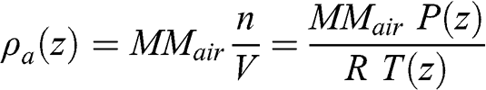
where z is altitude (m), P is pressure (here in Pa, i.e., kg m−1 s−2), ρa is the density of the air (kg m−3), and g is the gravitational constant (9.81 m s−2). For an incompressible fluid: ρa(z) = constant; therefore, the relationship between pressure and altitude is linear. For example, pressure increases almost linearly with depth in the oceans (with small variations due to changes in temperature and salt-content and a slight compressibility at very high pressure). The atmosphere is a gas and, therefore, a compressible fluid, implying that its density increases with pressure. The density of the air may be calculated according to the ideal gas law as follows:
 (3.3)
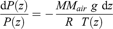
(3.3) where MMair is the average molar mass of the air, i.e., a weighted average of the molar masses of the various constituents of the air (0.029 kg mole−1 for dry air). Therefore, the dry air density is 1.184 kg m−3 at 1 atm and 25 °C; it is 1.225 kg m−3 at 1 atm and 15 °C. Replacing ρa(z) in the hydrostatic equation leads to:
 (3.4)
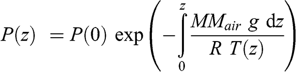
(3.4) Thus:
 (3.5)
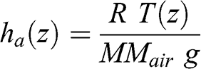
(3.5) This equation may be written as a function of a characteristic height, ha(z):
 (3.6)
(3.6) 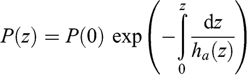 (3.7)
(3.7) This characteristic height varies as a function of altitude since temperature varies as a function of altitude. However, the variation of atmospheric temperature (expressed here in K) as a function of altitude is significantly less than that of pressure. If one assumes that temperature is constant, atmospheric pressure may then be written as a decreasing exponential function:
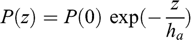 (3.8)
(3.8) where ha ≈ 8 km for a temperature of 273 K and R = 8.314 J mol−1 K−1. Thus, atmospheric pressure is about 0.88 atm at an altitude of 1 km and 0.29 atm at an altitude of 10 km. Figure 3.1 depicts this variation of atmospheric pressure with altitude.
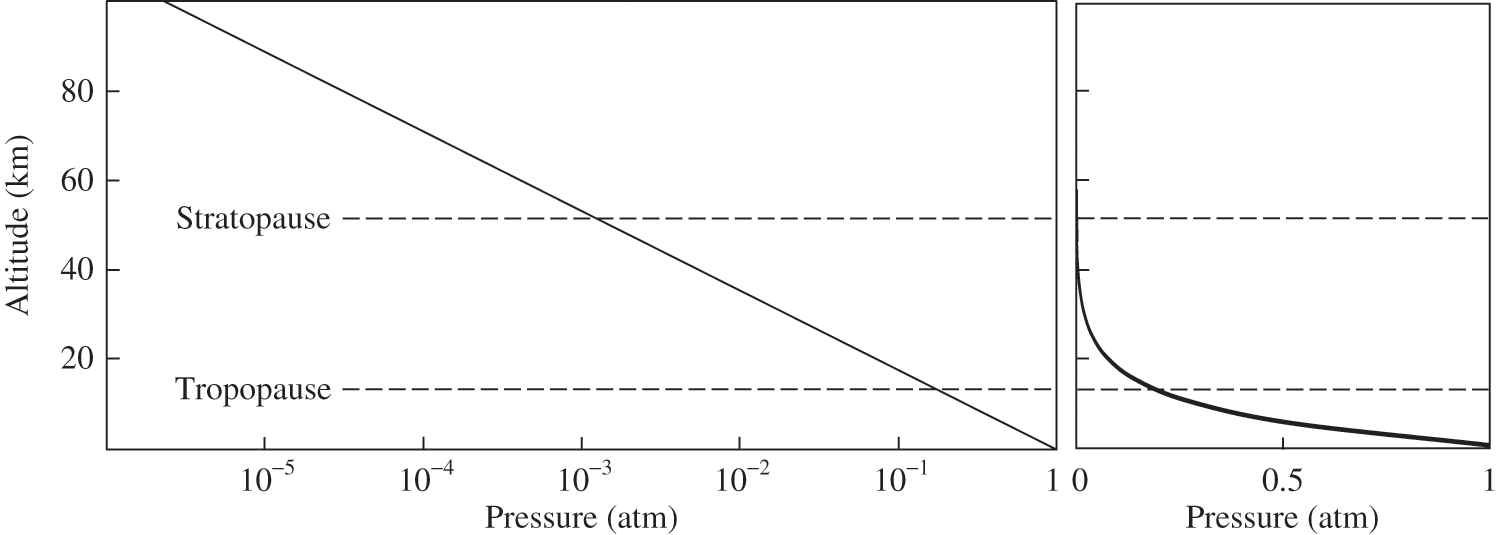
Figure 3.1. Vertical profile of atmospheric pressure. Atmospheric pressure is shown as a function of altitude with a logarithmic scale (left figure) and a linear scale (right figure). The tropopause and stratopause altitudes are approximate and given only as qualitative information.
The assumption of a quasi-constant temperature is in part justified by the fact that absolute temperature does not vary as much as pressure if one assumes that atmospheric processes are adiabatic (see Section 3.1.3). For example, the relationship between temperature and pressure results in a change of only 3 % in temperature for a change of 10 % in pressure.
The concentration of air molecules may be calculated according to the ideal gas law. Therefore, for an atmosphere with a pressure of 1 atm and a temperature of 25 °C (i.e., 298 K), the molar concentration is as follows:
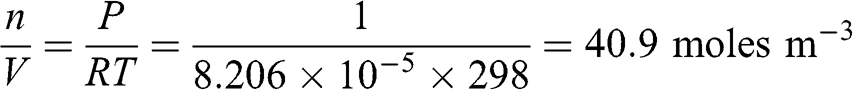 (3.9)
(3.9) The air density (ρa = MMair n / V) is proportional to its molar concentration; it increases proportionately with pressure and inversely proportionately with temperature (K). Therefore, warm air is less dense than cold air.
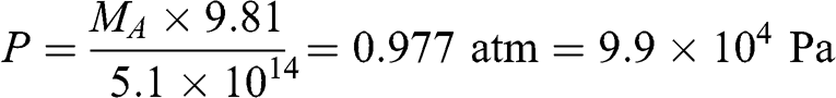
The unit of pressure “atmosphere” (atm) corresponds to the average atmospheric pressure observed at sea level at the latitude of Paris, France (≈ 49 °N). It varies at the Earth’s surface depending on altitude and temperature. For a given location, atmospheric pressure varies slightly, by a few % (see the discussion of high and low pressure systems as part of the general circulation description in Section 3.2.3). On average, it is 0.977 atm at the Earth’s surface because of altitude. Atmospheric pressure may be expressed with different units. For a reference pressure of 1 atm: P = 1 atm = 1.013 × 10⁵ Pa = 1,013 mbar (millibar) = 1,013 hPa (hectopascal) = 760 Torr (or mm of mercury).
The total mass of the Earth’s atmosphere, MA, may be calculated according to the definition of pressure being the force exerted by the atmosphere (i.e., the mass of the atmosphere multiplied by the acceleration of gravity) per unit surface area. The Earth’s surface area is 5.1 × 10⁸ km2, i.e., 5.1 × 10¹⁴ m2. Therefore, the corresponding pressure expressed in pascal (i.e., N m−2 or kg m−1 s−2) is:
 (3.10)
 Thus: MA = 5.15 × 10¹⁸ kg.
3.1.3 Vertical Structure of the Atmosphere
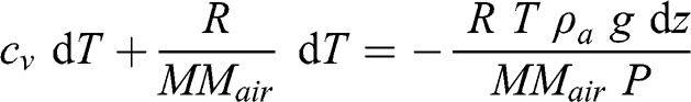
The temperature vertical profile may be derived from the first principle of thermodynamics and from the ideal gas law, with the assumption that the atmosphere is adiabatic. The first principle of thermodynamics may be written as follows:
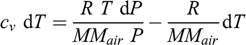
where the first term, dU, represents the change in the internal energy of the system (expressed here per mass, J kg−1), dQ (J kg−1) represents the amount of heat added to the system, and dW (J kg−1) represents the amount of work done by the system (or on the system if dW <0). For an adiabatic process, dQ = 0. Furthermore, for a parcel of air moving vertically, the expression for an ideal gas leads to:
where cv is the specific heat capacity of the air at constant volume (J kg−1 K−1):
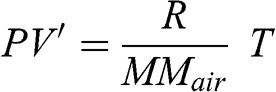
where V’ is the specific volume (i.e., the volume of an air parcel of 1 kg), which is equivalent to the inverse of the air density (V’ = V / (n MMair)), where MMair is expressed here in kg mole−1. Therefore:
It is more convenient to use only T and P as state variables and V’ may be replaced as a function of T and P. The ideal gas law may be written as a function of the specific volume:
 (3.15)
 By derivation:
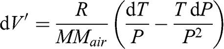 (3.16)
 Thus:
 (3.17)
 To obtain the vertical profile of temperature, one changes dP to dz according to the hydrostatic relationship (see Equation 3.2):
 (3.18)
 Substituting ρa as a function of P, T, and MMair (see Equation 3.3):
 (3.19)
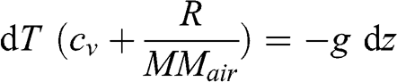
 Given that cp = (cv + (R/MMair)), where cp is the specific heat capacity at constant pressure:
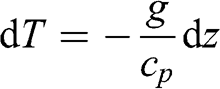 (3.20)
 Thus, for a given altitude difference:
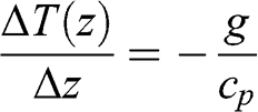 (3.21)
 Therefore, the adiabatic vertical gradient of the atmospheric temperature is linear. Given cp ≈ 1,000 J kg−1 K−1, the temperature gradient is −9.8 K km−1. This gradient corresponds to a dry atmosphere, i.e., without any water vapor. An adiabatic change with water vapor will affect temperature differently (see Chapter 4.2). As a result, the temperature adiabatic gradient for a wet atmosphere is less than that of a dry atmosphere. It is on average −6.5 K km−1; it is less in regions with high humidity (for example, in the tropics) and it tends toward the dry adiabatic gradient in regions with low humidity (for example, in deserts).
Near the Earth’s surface, the atmosphere is influenced by heat transfer between the surface and the atmosphere, as well as by turbulence generated by obstacles (e.g., vegetation, buildings, complex terrain). Therefore, the temperature vertical profile is not necessarily adiabatic (see Chapter 4.2). This part of the troposphere that is affected by the Earth’s surface is called the planetary boundary layer (PBL). The part of the troposphere located above the PBL is called the free troposphere. The troposphere corresponds to about ¾ of the total mass of the atmosphere. In the stratosphere, i.e., the atmospheric layer just above the troposphere, the strong absorption of ultraviolet radiation by oxygen and ozone (see Chapter 7) leads to an increase in temperature and the temperature vertical profile increases with altitude. The boundary between the troposphere and the stratosphere is called the tropopause. It may be defined in several ways:
– Thermal definition: the altitude at which the temperature vertical profile starts to increase
– Chemical definition: the altitude at which the ozone concentration starts to increase
– Dynamic definition: the altitude at which the dynamic vertical motions (characterized by the value of the potential vorticity, a variable that combines a representation of the dynamics of the flow and of the thermal stratification) decrease
These three processes (thermal, chemical, and dynamic) are related: the presence of oxygen leads via the absorption of solar radiation to the formation of ozone and an increase in temperature, and this temperature increase reduces vertical air motions (see Chapter 4). However, these definitions lead to slightly different values of the altitude of the tropopause. The definition of the tropopause by the World Meteorological Organization (WMO) is the lowest altitude at which the temperature decreases by less than 2 °C per km (and does not exceed this value on average for the next 2 km). An appropriate chemical definition is a value of 2.5 × 10⁻⁷ kg of ozone per kg of air, i.e., about 0.15 ppm for dry air. An appropriate dynamic definition is a value of the potential vorticity of 1.5 to 2 PVU (“Potential vorticity unit,” 1 PVU = 10−6 K m2 kg−1 s−1).
The atmosphere may be seen as comprising several layers of different properties. The troposphere ranges from the Earth’s surface to the tropopause. The altitude of the tropopause varies in space and time. It is greater at the equator (up to 17 km) and lower at the poles (about 7 km). Long-haul commercial flights take place at about 10 km altitude, i.e., in the upper troposphere. Supersonic commercial aircraft, such as Concorde, used to cruise in the stratosphere.
The stratosphere is generally defined as the atmospheric layer where temperature increases with height. Continuing upward, eventually the oxygen and ozone concentrations become too low to lead to any significant warming of the air, and temperature starts to decrease with altitude. This, the stratopause, occurs at about 50 km in altitude. The next layer is called the mesosphere.
The mesosphere ranges up to an altitude of about 85 km. The atmospheric layer above it is called the thermosphere (it includes the ionosphere where solar radiation leads to ionizing reactions producing gaseous ions). The thermosphere ranges up to about 500 to 1,000 km altitude. Beyond the thermosphere are the exosphere and the magnetosphere. The boundary between the atmosphere and outer space is generally considered to be at about 100 km altitude, at what is called the Kármán line. Here, the density of the atmosphere has become very low; it no longer behaves as a fluid and is not suitable for aeronautics. Beyond this boundary, gas molecules have few interactions among each other and those molecules that have enough kinetic energy may escape the Earth’s gravitational field and move into outer space.
Figure 3.2 depicts the average temperature vertical profile in the atmosphere, except for the planetary boundary layer. Near the Earth’s surface, the air temperature is affected by the surface and its vertical profile is not necessarily adiabatic (see Chapter 4).
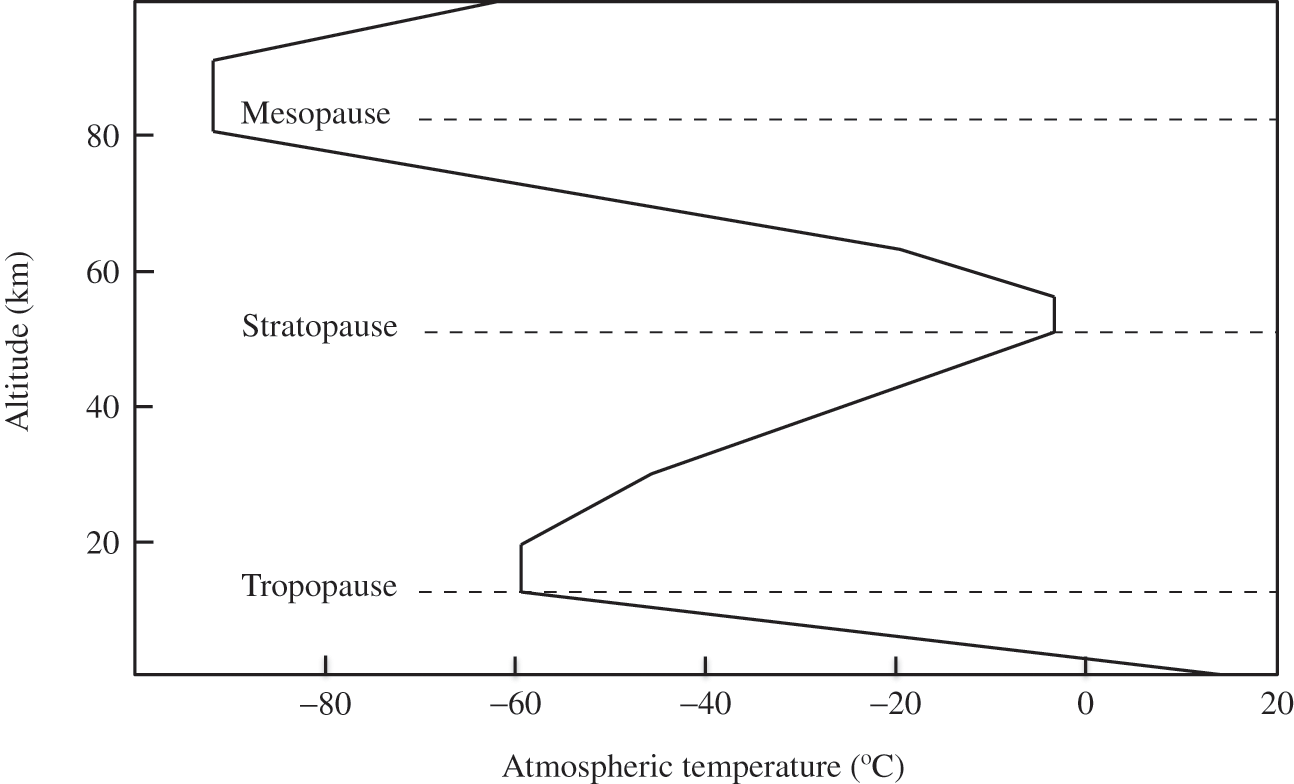
Figure 3.2. Typical vertical profile of the atmospheric temperature.
The mean radius of the Earth is 6,371 km. However, the Earth is not a perfect sphere as it is slightly flatter at the poles. Its radius varies from 6,378 km at the equator to 6,357 km at the poles. The atmosphere represents a fine layer surrounding this sphere. It corresponds to a thickness less than 2 % of the radius of the Earth if one considers the Kármán line and less than 1 % if one only includes the troposphere and stratosphere. The Earth’s surface is located entirely within the troposphere since the highest peaks of the Himalayas reach altitudes only slightly above 8,800 m. In terms of the atmospheric environment, i.e., the processes that affect the Earth’s surface and the impact of human activities on the atmospheric environment, it is sufficient to focus on the troposphere and the stratosphere.
3.1.4 Scales of Atmospheric Phenomena
Atmospheric phenomena cover a wide range of spatial and temporal scales, and it is useful to present briefly the concept of atmospheric scales and the corresponding phenomena.
The planetary scale corresponds to phenomena that cover important parts of the Earth and have temporal characteristics that are either permanent (or semi-permanent) or periodic. This category includes phenomena that constitute the general circulation (described in Section 3.2), as well as seasonal phenomena that recur every year, such as weather regimes (described in Section 3.3) and the monsoon.
The synoptic scale covers areas ranging from a few hundreds to several thousands of kilometers and time periods of several days. Major synoptic phenomena include low-pressure systems and high-pressure systems.
The mesoscale covers regional phenomena, which are affected by the regional physiographic configuration (coastal areas, mountainous areas, etc.). It ranges from a few kilometers up to the synoptic scale (i.e., several hundreds of kilometers). The corresponding time scales range from a few minutes up to one or two days. One may distinguish several subcategories of the mesoscale, which are, starting from the synoptic scale, the alpha mesoscale (approximately from 200 to 2000 km and from 6 h to 2 days), which covers part of the synoptic scale, the beta mesoscale (approximately from 20 to 200 km and from 30 min to 6 h), and the gamma mesoscale (approximately from 2 to 20 km and from 2 to 30 min). Examples of mesoscale meteorological phenomena include tropical storms at the alpha mesoscale, land/sea breezes and mountain/valley breezes at the beta mesoscale, and thunderstorms at the gamma mesoscale.
The aerologic scale (sometimes called the misoscale) covers areas ranging from a few hundred meters to several kilometers, with time scales on the order of a few minutes to an hour. Characteristic phenomena include tornadoes and isolated thunderstorms.
Finally, the microscale (which may include the misoscale) includes phenomena at the scale of a cloud or an eddy. Therefore, the corresponding areas may range from a few tens of centimeters to several hundreds of meters and the timescales range from a few seconds to several tens of minutes.
Note that the phenomena included in those different categories are related and that these scales are, therefore, interrelated. Furthermore, the spatial and temporal scales mentioned earlier in this section are approximate, because there is a large variability among the spatio-temporal characteristics of meteorological phenomena.
3.2 General Atmospheric Circulation
3.2.1 General Considerations
The general atmospheric circulation is governed by four major factors:
Solar radiation is more important at the equator than at the poles. Therefore, the amount of incoming energy absorbed by the Earth and its atmosphere is greater at the equator than at the poles. Furthermore, a lesser fraction is sent back into space from the tropics than from higher latitudes because of water vapor that is present, on average, in larger amount in the tropical atmosphere than at other latitudes. In addition, snow and ice, which are ubiquitous in the polar regions, lead to more radiation being reflected by the Earth’s surface and, therefore, less absorption of radiative energy at the poles and in boreal regions than in the tropics. These phenomena, which are related mostly to the water cycle (evaporation in the tropics with the associated cloud formation and latent heat, presence of ice and snow in the polar regions) lead to a thermal energy difference between the equator (or more generally the tropics) and the polar regions. On average, the Earth is at equilibrium and a transfer of heat from the equator toward the poles must occur to prevent an accumulation of heat at the equator and a depletion at the poles (see Chapter 5).
The presence of oxygen in the Earth’s atmosphere leads to the absorption of ultraviolet radiation by oxygen and ozone molecules in the stratosphere. These phenomena are described in Chapter 7. This absorption of radiative energy leads to a temperature increase in the stratosphere and, consequently, an inversion of the vertical temperature gradient above the tropopause. Such a temperature inversion leads to a quasi suppression of vertical motions of air parcels through the tropopause region (see Chapter 4).
The rotation of the Earth leads to a deviation of the atmospheric flow toward the right in the northern hemisphere and toward the left in the southern hemisphere. These deviations result from the Coriolis force, which is explained next.
3.2.2 Coriolis Force
The Earth’s rotation leads to the fact that an air parcel moving along one direction in a space-fixed coordinate system will move along a different trajectory seen from an Earth-based rotating coordinate system. A simple demonstration consists in following the trajectory of an air parcel in the northern hemisphere that is moving southward. Let us assume that for an observer in a space-fixed coordinate system, the initial motion of this air parcel follows a straight-line trajectory, i.e., along a meridian (meridional trajectory, which has a constant longitude) and moves for a time step ∆t from a high latitude, ϕ1, toward a lower latitude, ϕ2. If the Earth’s rotation (angular velocity) is ΩT, at ∆t the meridian is located east of its initial location in a space-fixed coordinate system at a zonal distance (i.e., along its new latitude ϕ2): ∆x2 = ΩT rT cos(ϕ2) ∆t, where rT is the mean radius of the Earth. On the other hand, the air parcel has moved along a trajectory that corresponds to its initial velocity, ΩT rT cos(ϕ1), and the zonal distance between the location of the air parcel and its initial location is ∆x1 = ΩT rT cos(ϕ1) ∆t. Since the air parcel is moving southward toward the equator: ϕ1 > ϕ2, therefore, cos(ϕ1) < cos(ϕ2). Thus, the air parcel is slightly behind the meridian corresponding to its initial location after the time step ∆t (∆x1 < ∆x2). Figure 3.3 illustrates this example.
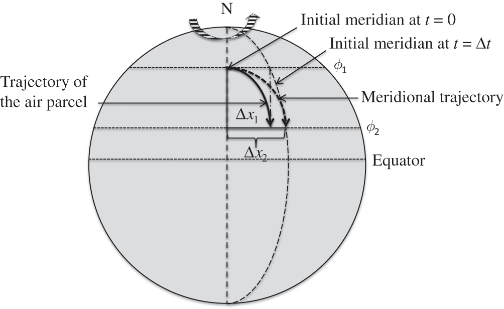
Figure 3.3. Schematic representation of the Coriolis force. The effect of the Earth’s rotation is shown for a southward meridional atmospheric flow in the northern hemisphere.
Conversely, if the air parcel trajectory moves northward in the northern hemisphere, ϕ1 < ϕ2, and therefore, cos(ϕ1) > cos(ϕ2). Then, the air parcel is slightly ahead of the initial meridian after a time step ∆t (∆x1 > ∆x2). In both cases, the air parcel trajectory has been deviated toward the right. The same demonstration can be carried out for the southern hemisphere, where the air parcel trajectory will be deviated to the left.
This conceptual description of the effect of the Earth’s rotation on the direction of the atmospheric flow is actually approximate. Indeed, according to this demonstration, the motion of an air parcel along a latitude (zonal trajectory), for example eastward, would not lead to any deviation. Nevertheless, the Earth’s rotation affects also air parcels with zonal trajectories and the associated deviations are also toward the right in the northern hemisphere and toward the left in the southern hemisphere.
The deviations of the atmospheric flow toward the right in the northern hemisphere and toward the left in the southern hemisphere result from a virtual force called the Coriolis force after Gustave-Gaspard Coriolis, who formulated its mathematical representation in 1835 (it had been identified as early as in the 17th century concerning the trajectories of cannon balls by Riccioli and Grimaldi). The Coriolis force is zero at the equator and is maximum at the poles.
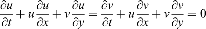
The acceleration of the flow velocity may be defined simply according to the Navier-Stokes equations of fluid mechanics (see Chapter 4 for a more complete description of these equations). Here, we ignore the vertical wind velocity, which is typically negligible compared to the horizontal components:
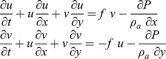 (3.22)
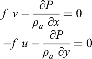
 where f is the Coriolis parameter: f = 2 ΩT sin(ϕ), where ΩT is the angular velocity of the Earth (radian s−1) and ϕ is the latitude (°). The terms on the left-hand side correspond to the total derivative of the components of the horizontal wind velocity. The first terms on the right-hand side correspond to the Coriolis force and the second terms correspond to the pressure gradient force. At equilibrium (i.e., without any acceleration):
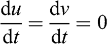 (3.23)
 Changing total derivatives into partial derivatives:
 (3.24)
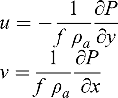
 Therefore, the atmospheric flow is given by the following equations:
 (3.25)
 These equations correspond to the geostrophic wind, i.e., the case where there is equilibrium between the pressure gradient force and the Coriolis force. Therefore:
 (3.26)
 In the very simple case of the general circulation described in Section 3.2.3, the atmospheric pressure gradients are along the meridians, therefore: ∂P / ∂x = 0. Then:
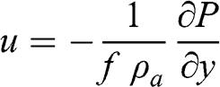 (3.27)
 The pressure gradient between a latitude of 30 °N (high-pressure region) and a latitude of 60 °N (low-pressure region) is negative (see Section 3.2.3). Therefore, u is positive, which corresponds to mid-latitude winds blowing eastward (i.e., westerly winds). This simple calculation does not account for the complexity of atmospheric motions, which (1) are not at equilibrium and (2) include a vertical component. Furthermore, the Coriolis parameter tends toward 0 when the latitude tends toward zero (at the equator); therefore, this calculation is not strictly applicable in the tropics.
3.2.3 Conceptual Representation of the Atmospheric General Circulation
The heat excess at the equator and the heat deficiency at the poles lead to a circulation transferring this heat from the tropics toward the polar regions (see Chapter 5). At the equator, the heat excess leads to a less dense atmosphere (according to the ideal gas law) and, therefore, an upward air motion toward the tropopause. This upward motion leads to a low pressure at the surface. The upward motion stops at the tropopause since the temperature inversion creates a stable layer, which tends to suppress vertical air motions. An air parcel moving upward must then move away from the equator toward the tropics. The Coriolis force deviates this air parcel eastward. Once its motion toward the poles has slowed down sufficiently (at about 30 °N and 30 °S), it cannot remain at the same altitude, because the space east of its position is already occupied by another air parcel; therefore, it must subside. This subsidence leads to high-pressure regions in the subtropical regions. The cycle is completed when air from the high-pressure regions moves toward the low-pressure region at the equator. This cycle was proposed by George Hadley, who was an attorney and amateur meteorologist. Accordingly, these atmospheric circulations are called the Hadley cells. The high-pressure regions, which are at about 30 °, are characterized by little rain and as a result many of the world deserts are located at those latitudes: for example, the Sahara desert in Africa, the Sonora desert in North America, the Arabian desert in Asia, and the Victoria desert in Australia.
A cycle similar to that of the Hadley cells occurs in the polar regions. These polar cells result from a subsidence of cold and dry air over the poles. At the surface, this descending air must move toward lower latitudes. At latitudes around 60 °, these air parcels run into air parcels that move toward higher latitudes from the high-pressure subtropical regions. Thus, an ascending motion occurs around 60 °. At these latitudes, the ascending air parcels lead to water vapor condensation and, therefore, heavy precipitation. These regions are associated with polar fronts. The upward air parcels meet the tropopause, but at altitudes lower than at the equator. These air parcels move then toward the poles where they subside, or toward lower latitudes where around 30 ° they meet air parcels originating from the equator.
The Hadley cells do not transfer energy from the equator to the poles because the air parcels subside and return toward the equator in the subtropical regions. The transfer continues in the temperate regions, i.e., the mid-latitudes, with a cycle that ranges from about 30 ° to 60 °. Those are the Ferrel cells. The transfer is completed with the polar cells, which move air parcels toward the poles via the ascending air motions at about 60 °.
Schematically, there is a low-pressure region at the equator and, in both hemispheres, a high-pressure region at about 30 °, a low-pressure region at about 60 °, and high-pressure regions at the poles. In the northern hemisphere, these high- and low-pressure regions are mostly limited to the oceans, because the presence of land masses affects these flow cycles significantly. Semi-permanent high-pressure regions around 30 ° include the Bermuda High in the Atlantic Ocean and the Pacific High in the Pacific Ocean. Semi-permanent low-pressure regions around 60 ° include the Aleutian Low in the Pacific Ocean and the Icelandic Low in the Atlantic Ocean. On the other hand, in the southern hemisphere, where land masses are few, there are three major high-pressure regions in the Atlantic, Indian, and Pacific Oceans, which are better defined than those of the northern hemisphere. There is also a low-pressure belt at about 60 °. On land, low- and high-pressure regions occur due to phenomena related to energy balance and atmospheric flows specific to land masses (for example, the Siberian High). The geographical locations of these low- and high-pressure regions vary according to season, since the energy balance depends on solar radiation. For example, the Pacific and Bermuda Highs are present at lower latitudes in winter than in summer.
The atmospheric flow occurs from high-pressure regions toward low-pressure regions, i.e., from latitudes of about 30 ° toward the equator (subtropical and tropical regions) and toward higher latitudes of about 60 ° (temperate regions) and from the poles toward the 60 ° latitudes (polar and subpolar regions). The Coriolis force affects these air flows, which initially are meridional flows (i.e., along a meridian).
In the subtropical and tropical regions, the air flowing toward the equator will be deviated toward the right in the northern hemisphere and toward the left in the southern hemisphere, i.e., westward. Thus, the winds in those regions are mostly easterly (i.e., originating from the east; more precisely northeasterly winds in the northern hemisphere and southeasterly winds in the southern hemisphere). They are typically called the trade winds, because they favored trade with ships sailing between Europe and the American continents. In the temperate regions, the deviation of winds toward the right in the northern hemisphere and toward the left in the southern hemisphere leads to prevailing winds originating mostly from the southwest in the northern hemisphere and from the northwest in the southern hemisphere. In the polar regions, the air flows originating from the poles are deviated westward. Figure 3.4 summarizes schematically these main aspects of the atmospheric general circulation. More detailed descriptions are available in the scientific literature (for example, James, 1994).
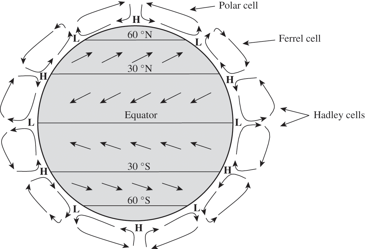
Figure 3.4. Atmospheric general circulation. This simplified representation depicts schematically the Hadley cells in the subtropical and tropical regions, the Ferrel cells in the temperate regions, the polar cells, the prevailing westerly winds in the mid-latitudes, and the easterly trade winds in the tropical regions. The semi-permanent high-pressure regions (H) are mostly at about 30 ° latitude and at the poles; the semi-permanent low-pressure regions (L) are mostly at 60 ° latitude.
3.3 Meteorological Regimes
3.3.1 Main Regimes
The processes described in Section 3.2 represent a very simple overview of the general atmospheric circulation. As mentioned, the main characteristics of this general circulation occur over the oceans and little over the continents. Indeed, the presence of complex terrain modifies the heat exchanges and atmospheric flows. Furthermore, the chaotic nature of meteorology implies that a small difference in an initial state of the atmosphere can lead to significant differences a few days later. Therefore, within the conceptual representation presented in Section 3.2, several scenarios may develop in relation with permanent structures (e.g., the Hadley cells) and semi-permanent ones (e.g., the Bermuda High and the Icelandic Low in the case of Europe; the Pacific High and the Aleutian Low in the case of North America). These meteorological scenarios are nevertheless limited in terms of their main characteristics, and they can be grouped in several regimes. For example, a representation using four meteorological regimes per season (i.e., 16 weather regimes in total) can be used for Europe. All days of a meteorological regime are not identical; however, they share similar characteristics at the synoptic scale. Figure 3.5 summarizes such a classification for the northern Atlantic Ocean and Europe for winter (December to February) and summer (June to August). These maps represent pressure anomalies compared to means calculated from meteorological data over the period 1950–2008. The frequencies of each regime are shown. Transition days lead to the change from one regime to the next. However, all regimes do not necessarily evolve into all other regimes. Spring and fall can also be represented with such regimes, which are intermediate between those of winter and summer.
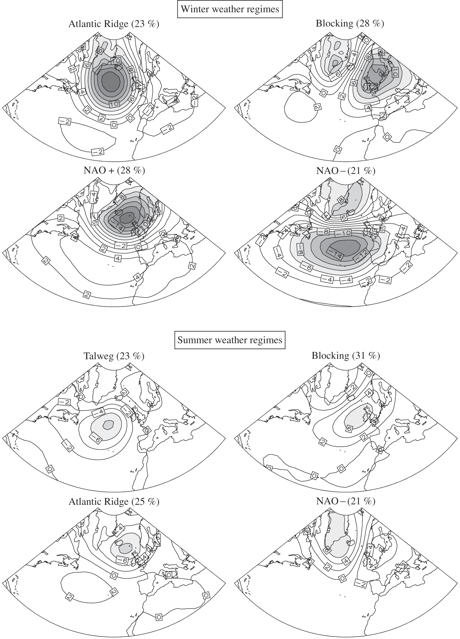
Figure 3.5. Weather regimes over the North Atlantic in winter (top figure) and summer (bottom figure). The occurrence frequencies for the period 1950–2008 are shown in terms of anomalies in the atmospheric pressure at sea level (PSL, hPa) with respect to the seasonal mean. Winter corresponds to December-January-February and summer corresponds to June-July-August.
The meteorological regimes called “North Atlantic Oscillation” (NAO) correspond to variations in the atmospheric pressure between the Bermuda High (as measured in Lisbon) and the Icelandic Low (as measured in Reykjavik). The NAO+ regime corresponds to periods when the pressure difference between these two locations is greater than the mean and the NAO- regime corresponds to the opposite situation. The Atlantic Ridge regime corresponds to a high-pressure region (barometric ridge) that originates from the Bermuda High and spreads northward over the Atlantic Ocean. Similarly, the Atlantic Talweg regime corresponds to a low-pressure region (barometric valley) that originates from the Icelandic Low and spreads southward over the northern Atlantic Ocean. The blocking regimes correspond to high-pressure and low-pressure regions that are stationary with respect to one another and, therefore, lead to meteorological conditions over the corresponding regions that vary little during the period of the blocking regime.
Weather regimes have similarly been developed for other world regions. For example, Robertson and Ghil (1999) used six regimes to characterize meteorology during winter over the western United States.
3.3.2 Fronts and Blocks
A front is a virtual surface between two air masses of different properties (in terms of temperature, humidity, and pressure). One typically distinguishes cold fronts and warm fronts.
In a cold front, a cold air mass moves toward a warm air mass. Since the cold air is denser than the warm air, the cold air mass moves underneath the warm air mass, thereby lifting the warm air mass. The humid warm air encounters lower temperature aloft, which leads to the formation of clouds ahead of the cold front.
In a warm front, a warm air mass moves toward a cold air mass. The warm air is less dense than the cold air; therefore, the warm air mass moves on top of the cold air mass. Then, clouds form over the cold air mass.
One also considers stationary and occluded fronts. A stationary front corresponds to a virtual surface separating two air masses, one cold and the other warm, that are nearly stationary with respect to each other (for example, in the case where wind directions are parallel to the front). An occluded front corresponds to the case where a cold front catches up with a warm front. Then, the warm air mass is lifted above both cold air masses surrounding it.
Fronts are associated with precipitations, which result from the cloud formation in the frontal zone. These precipitations scavenge atmospheric pollutants (see Chapter 11) and a frontal situation is generally associated with an improvement in air quality.
A block results from the interruption of the zonal circulation in the mid-latitudes. This interruption is due to the presence of a high-pressure system (or that of a low-pressure system), which deviates the prevailing winds toward the north (or the south) in the northern hemisphere. In Europe, the blocking regimes correspond to the presence of a high-pressure system located over western Europe. Such a blocking regime may last several days and leads in the high-pressure region to meteorological conditions characterized by low wind speeds and clear skies. These conditions are conducive to an increase of the air pollution because of a reduced dispersion of the pollutants and the increased formation of secondary pollutants due to photochemical reactions enhanced by the increased solar radiation (see Chapters 6, 8, and 9).
Examples: Air pollution episodes in the Paris region
The two selected air pollution episodes occurred in the Paris region in December 2013 (winter conditions) and March 2014 (spring conditions). A meteorological analysis was conducted by Météo France, the French national weather service, for these episodes (see Figure 3.6, Tonnelier et al., 2015).
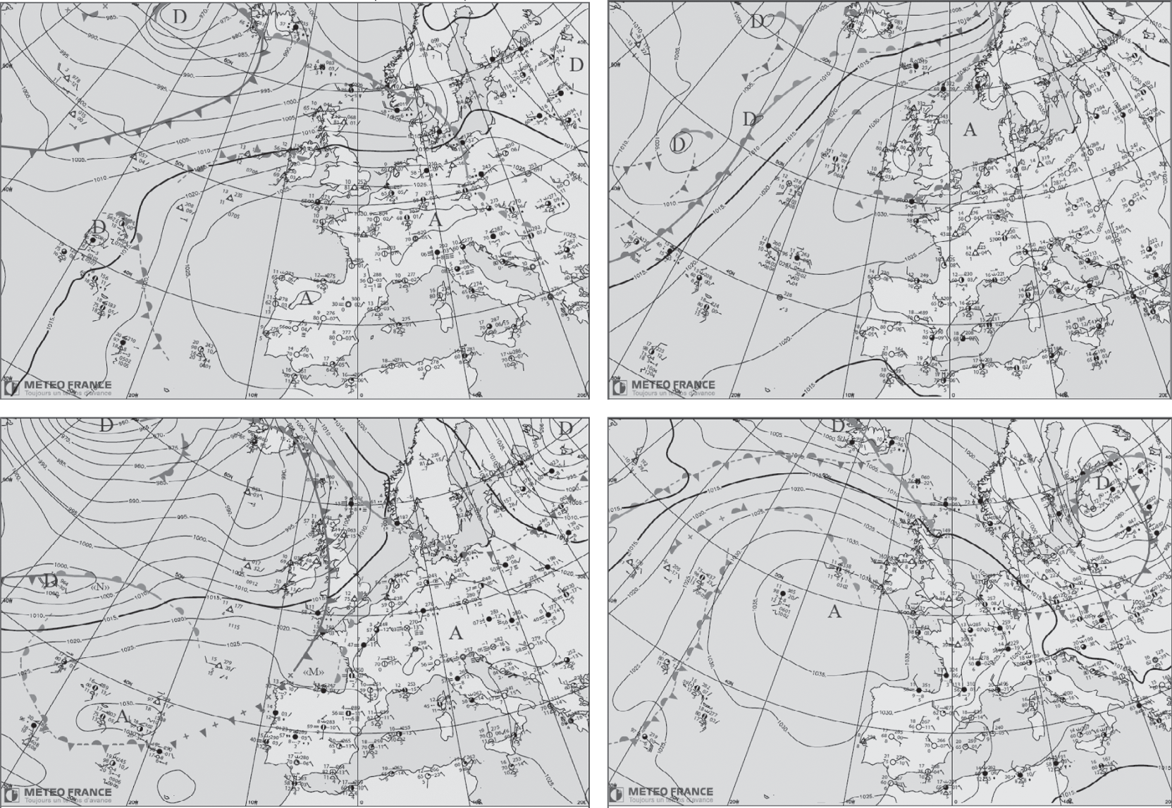
Figure 3.6. Meteorological conditions of air pollution episodes over the Paris region. Left figures: meteorological conditions of a winter air pollution episode dominated by primary PM on December 8, 2013 (top figure) and on December 13, 2013 (bottom figure, end of the episode); right figures: meteorological conditions of a spring air pollution episode dominated by secondary PM on March 11, 2014 (top figure) and on March 15, 2014 (bottom figure, end of the episode). “A” stands for “anticyclone” (i.e., high-pressure system); “D” for “depression” (i.e., low-pressure system).
The episode occurring from December 8 to 12, 2013 corresponds to air pollution dominated by primary particulate matter (PM), i.e., those atmospheric particles that are directly emitted into the atmosphere (see Chapter 9). The PM10 hourly concentrations exceeded 100 μg m−3 and the black-carbon hourly concentrations (mostly emitted by diesel vehicles and biomass combustion) reached 12 μg m−3. On December 8, a high-pressure system covered western Europe (1025 to 1035 hPa) and low-pressure regions were present over the northern Atlantic. These conditions correspond to a blocking regime (see Figure 3.6). The prevailing winds over the Paris region were from the southeast with low wind speeds. A strong temperature inversion was present in the planetary boundary layer, not only at night, but also during the day because of the low wintertime solar radiation. The temperature varied between −2 and 8 °C. This episode ended on December 13, with the end of the blocking regime and a transition toward a regime with westerly winds, which brought maritime air masses. This new NAO+ regime was then characterized by low-pressure systems coming from the northern Atlantic and a high-pressure region centered over the Atlantic south of Spain.
The episode occurring from March 11 to 14, 2014 corresponds to air pollution with PM10 hourly concentrations exceeding 160 μg m−3. Unlike the winter episode mentioned, this spring episode was dominated by the secondary fraction of PM, which results from the condensation of semi-volatile compounds formed in the atmosphere via photochemical reactions of gaseous pollutants (see Chapter 9). These reactions were enhanced by a strong springtime solar radiation and clear skies. The meteorological conditions correspond to a blocking regime with a high-pressure system over western Europe (1025 to 1030 hPa) and low-pressure systems over the northern Atlantic. In the Paris region, low wind speeds followed the moderate wind speeds of the previous days with prevailing northeastern wind directions. The temperature inversion that was present at night remained in the morning, but disappeared during the day due to strong solar radiation. The temperature varied between 8 and 20 °C. The moderate temperature during the day favored chemical kinetics leading to the formation of nitric acid and semi-volatile organic compounds (SVOC) via oxidation of gaseous precursors. On the other hand, the low nighttime and morning temperature favored the condensation of these semi-volatile compounds on existing particles and, therefore, the formation of a significant secondary PM fraction (ammonium nitrate and secondary organic aerosols). This episode ended in a manner similar to that of the other one mentioned, i.e., via the arrival of maritime air masses. However, the transition was less pronounced than for the winter episode, because the high-pressure system located over the Atlantic Ocean was still present in the vicinity of France, i.e., at a higher latitude than in winter.
Problems
Problem 3.1 Calculation of atmospheric pressure
Calculate the atmospheric pressure and temperature at an altitude of 5 km, given that atmospheric pressure and temperature at sea level are 1 atm and 20 °C, respectively, and that atmospheric conditions are dry.
Problem 3.2 Coriolis force
a. Calculate the Coriolis parameter at a latitude of 45 °.
b. Compare at that latitude the accelerations due to a pressure gradient of 8 mbar over a distance of 400 km and the Coriolis force for a wind speed of 10 m s−1.
c. Calculate the geostrophic wind speed at that latitude and for this pressure gradient.