Abstract
Population exposure to air pollution occurs mostly near the Earth’s surface. Furthermore, most air pollution sources are located near the Earth’s surface (some exceptions include tall stacks, aircraft emissions, and volcanic eruptions). Therefore, the meteorological phenomena of the lower layers of the atmosphere are the most relevant to understand and analyze air pollution. The part of the atmosphere that is in contact with the Earth’s surface and is affected by it is called the atmospheric planetary boundary layer (PBL). This chapter describes the dynamic processes that take place within the PBL. Those include, in particular, turbulent atmospheric flows and heat transfer processes, which affect air pollution near the surface. Those processes are often referred to as “air pollution meteorology,” because they are the most relevant to air pollution. The major equations governing these processes are presented. A more detailed description of the PBL is available in books such as those by Stull (1988) and Arya (2001).
Population exposure to air pollution occurs mostly near the Earth’s surface. Furthermore, most air pollution sources are located near the Earth’s surface (some exceptions include tall stacks, aircraft emissions, and volcanic eruptions). Therefore, the meteorological phenomena of the lower layers of the atmosphere are the most relevant to understand and analyze air pollution. The part of the atmosphere that is in contact with the Earth’s surface and is affected by it is called the atmospheric planetary boundary layer (PBL). This chapter describes the dynamic processes that take place within the PBL. Those include, in particular, turbulent atmospheric flows and heat transfer processes, which affect air pollution near the surface. Those processes are often referred to as “air pollution meteorology,” because they are the most relevant to air pollution. The major equations governing these processes are presented. A more detailed description of the PBL is available in books such as those by Stull (1988) and Arya (2001).
4.1 The Atmospheric Planetary Boundary Layer
The PBL can be defined according to its dynamic or thermal processes. From a dynamic viewpoint, the PBL is the atmospheric layer that is affected by the Earth’s surface, either because of mechanical effects due to terrain, buildings, vegetation, etc., or indirectly because of heat transfer processes related to the evaporation of water or the anthropogenic production of heat (for example, the urban heat island effect). From a thermal viewpoint, the PBL is the atmospheric layer that is affected by the temporal variation of solar radiation, for example via its ambient temperature.
The PBL height varies as a function of terrain and solar radiation. It is on the order of a kilometer, but it is lower in winter when there is little solar radiation (on the order of a few hundred meters) and greater in summer when solar radiation is maximum (on the order of 2,000 to 3,000 m).
Within the PBL, one distinguishes the surface layer, which is located near the surface. Within the surface layer, vertical fluxes of momentum, heat, and mass transfer are nearly constant (~±10 %). The surface layer has a thickness that is less than 10 % of that of the PBL. One should note, however, that within a forest or an urban canopy, the atmospheric flows are generally complex and the vertical fluxes are most likely not constant.
Above the PBL, the effect of the Earth’s surface is negligible: this is the free atmosphere. When one is interested in air pollution at local or urban scales, it is generally appropriate to take into account only the PBL. On the other hand, when one is interested in air pollution at regional, continental, or global scales, the free troposphere must be taken into account, because air pollutants can be transported over long distances in the free troposphere and precipitation events, which scavenge air pollutants, generally include a significant fraction of the free troposphere.
4.2 Vertical Motions of Air Parcels
4.2.1 Potential Temperature
The change of pressure and temperature as a function of altitude is obtained via the hydrostatic and ideal gas laws (see Chapter 3). Furthermore, a relationship between pressure and temperature may be obtained by assuming that air parcels undergo adiabatic changes. Therefore, the law of Laplace applies:
where γ is the adiabatic index of the gas (here, air), also known as the Laplace coefficient (γ = cp / cv, where cp and cv are the specific heat capacities at constant pressure and volume, respectively). Applying the ideal gas law (see Chapter 3), the following relationship between pressure and temperature is obtained under adiabatic conditions:
For a diatomic gas (which is the case of the atmosphere, since molecular nitrogen and oxygen account for 99 % of the air), γ = 7/5 = 1.4. Thus:
Therefore:
The potential temperature, θ, is defined as the temperature of an air parcel brought back to sea level at a standard pressure (i.e., P0 = 1 atm) under adiabatic conditions. Therefore:
 (4.5)
(4.5) Thus:
 (4.6)
(4.6) 4.2.2 Neutral Atmosphere
A constant vertical profile of the potential temperature is defined as neutral. Let us consider an air parcel with uniform properties (pressure, temperature, and density). Under neutral conditions, this air parcel will remain in equilibrium with its environment as it moves upward or downward, since its temperature will change adiabatically and will, therefore, remain consistent with the temperature of the surrounding air.
4.2.3 Unstable Atmosphere
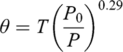
The atmosphere is unstable if the vertical profile of the potential temperature is negative, i.e., if the actual temperature decreases faster with height than the adiabatic gradient. An air parcel moving upward becomes warmer than that of its surroundings, because its adiabatic change in temperature is less than the decrease of the surrounding atmospheric temperature. Therefore, according to the ideal gas law, the density of this air parcel becomes less than that of the surrounding air. Thus, this air parcel keeps moving upward. Similarly, an air parcel moving downward undergoes an adiabatic change and its temperature change is less than that of the gradient of the surrounding atmosphere. Therefore, the surrounding temperature becomes greater than that of the air parcel. Thus, this air parcel is denser than the surrounding air and it continues to move downward. Vertical motions in an unstable atmosphere are enhanced because a small perturbation in the vertical direction leads to continuous motion in the direction of the initial perturbation (see Figure 4.1). Such unstable air parcels lead to vertical mixing of air pollution, at least up to an altitude where the atmosphere becomes neutral or stable (see Section 4.2.4). An unstable atmospheric layer is called a mixing layer. It occurs generally within the PBL during the day, because solar radiation warms up the Earth’s surface, but does not affect the temperature of the lower atmosphere (since the air absorbs little ultraviolet radiation within the troposphere, see Chapter 5). As a result, the vertical potential temperature gradient becomes negative.
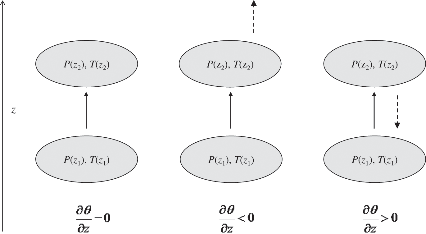
Figure 4.1. Schematic representation of vertical motions of an air parcel for neutral conditions (left figure), unstable conditions (middle figure), and stable conditions (right figure). The solid arrows indicate the initial perturbation of the air parcel, which undergoes an adiabatic change, and the dashed arrows indicate the following motion of the air parcel, which is due to the difference between the temperature of the air parcel and that of the surrounding air (i.e., density difference).
4.2.4 Stable Atmosphere
The atmosphere is stable if the vertical profile of the potential temperature becomes positive. As an air parcel moves upward, its temperature follows an adiabatic change and it becomes lower than that of the surrounding air. Therefore, the air parcel becomes denser than the surrounding air. As a result, it tends to move back downward. Similarly, an air parcel moving downward undergoes an adiabatic change and its temperature becomes greater than that of the surrounding air. Thus, this air parcel, being less dense than the surrounding air, tends to move back upward. Therefore, a stable atmosphere tends to suppress vertical motions of air parcels. Thus, such an atmospheric layer may become stratified, because there are no, or few, transfers between the different layers (strata) of the atmosphere (see Figure 4.1). A stable atmospheric layer may be present aloft, for example above a mixing layer, or at the surface. This latter case occurs at night when the infrared radiation emitted by the Earth’s surface toward the atmosphere leads to a decrease of the surface temperature and, accordingly, of the surface layer temperature. Therefore, a temperature inversion develops: the gradient of the actual temperature becomes positive and the gradient of the potential temperature becomes also positive. (Note that an atmospheric layer may be stable without a temperature inversion, as long as the actual temperature gradient is less than the adiabatic gradient.) Then, the atmospheric layer near the surface is stable at night. This stable layer will gradually become thicker as the surface temperature keeps decreasing. The PBL layer located above this stable layer is called the residual layer. Pollutants located within this residual layer are then isolated from the surface. However, during daytime, as solar radiation warms the surface, thereby leading to the gradual disappearance of the surface-based stable layer, the previously stable and residual layers merge to form a new mixing layer. Pollutants that were formerly present within the residual layer are mixed vertically and may then interact with the surface. The evolution of the atmospheric layer near the Earth’s surface is depicted schematically in Figure 4.2. The stratosphere shows a positive vertical profile of the potential temperature; therefore, it is a stable atmospheric layer with few vertical air motions.
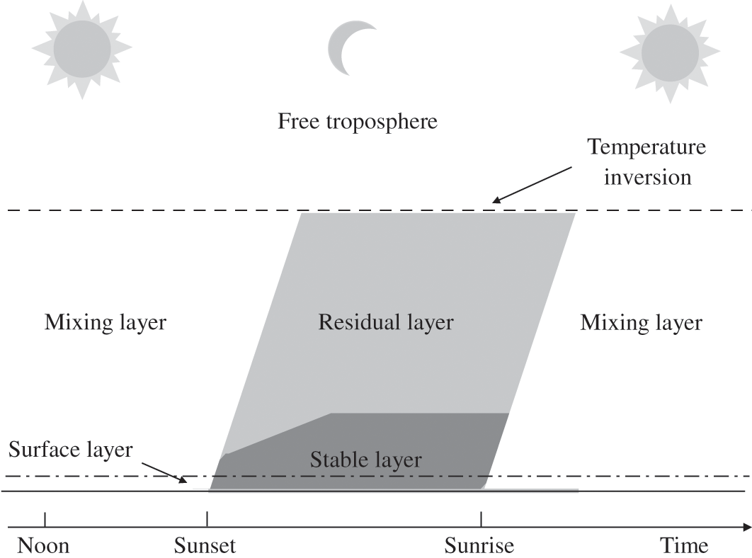
Figure 4.2. Schematic representation of the daily cycle of the planetary boundary layer.
4.2.5 Effect of Moisture
This description of temperature gradients applies to dry atmospheres. If the atmosphere is moist, its vertical temperature gradient under adiabatic conditions will be less than that of a dry atmosphere. The water content, q (i.e., the specific humidity expressed in g of water per g of moist air), corresponds to a relative humidity (%), which is greater when temperature decreases, because the saturation vapor pressure of water decreases with temperature. In other words, for a given quantity (mass) of water per quantity of air (mass or volume), relative humidity increases when temperature decreases. Accordingly, for a given relative humidity, the water content of the atmosphere decreases when temperature decreases.
Humidity
Relative humidity (%) may be converted to absolute humidity using the method proposed by McRae (1980). According to Dalton’s law, the water vapor concentration expressed in parts per million (ppm; 1 ppm = 1 molecule per million molecules of air) is:
 (4.7)
(4.7) where T is the ambient temperature, Ps,H2O(T) is the saturation vapor pressure of water, and P is the atmospheric pressure. The saturation vapor pressure of water depends on temperature according to the following polynomial formula:
 (4.8)
(4.8) where ωT = 1 – (373.15/T), where T is expressed in K. For example, at P = 1 atm and T = 25 °C, Ps,H2O (298 K) = 0.031 atm; at T = 5 °C, Ps,H2O (278 K) = 0.0086 atm. At a relative humidity of 50 % and a temperature of 5 °C, there are about 4300 ppm of water vapor.
Converting % to (g m−3) is performed as follows:
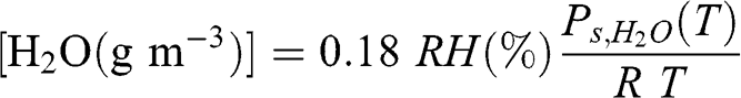 (4.9)
(4.9) Thus, a relative humidity of 50 % at 1 atm and 5 °C corresponds to 3.4 g of water vapor per m3 of air. The water vapor mass per volume of air is called the volumetric absolute humidity. The water vapor mass concentration at saturation (RH = 100 %) increases with temperature. For example, at 1 atm, there are 9.4, 17, and 30 g of water vapor per m3 at 10, 20, and 30 °C, respectively.
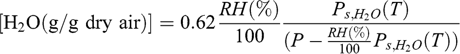
Absolute humidity may also be defined as the mass of water vapor per mass of air. It can be defined per mass of dry air or per mass of moist air. The absolute humidity per mass of dry air is usually called the mixing ratio (by weight) and the absolute humidity per mass of moist air is usually called the specific humidity. The molar mass of dry air is 29 g mole−1; therefore, according to the ideal gas law, the mass in g of one m3 of dry air is: 29 Pdry air /(RT). The mixing ratio is thus related to relative humidity as follows:
 (4.10)
 According to Dalton’s law, the total pressure is the sum of the partial pressures of dry air and water vapor:
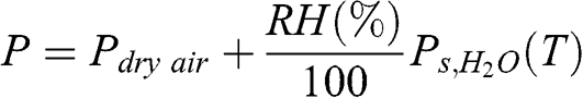 (4.11)
 Therefore:
 (4.12)
 The specific humidity, q, is related to relative humidity as follows:
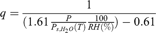 (4.13)
 Given that water vapor is a small fraction of the total mass of an air parcel, the mixing ratio and the specific humidity generally have very close values. For example, at T = 25 °C and P = 1 atm, Ps,H2O = 0.031 atm (see previous equation). For a relative humidity of 100 %, the mixing ratio is calculated to be 0.0198 g H2O/g dry air and the specific humidity, q, is 0.0195 g H2O/g moist air, i.e., a difference of less than 2 %.
Virtual Temperature
The virtual temperature of a moist air parcel, Tv, is defined as the temperature that dry air would have for the same values of pressure and density as moist air. The relationship between the actual temperature, T, and the virtual temperature, Tv, (in K) is a function of the specific humidity, q (g of water/g of moist air), of the air parcel. It is given approximately by the following formula (see, for example, Wallace and Hobbs, 2006, for the exact relationship and the derivation of this simplified relationship):
The ideal gas law applies to a moist air parcel if Tv is used instead of T. Since water vapor has a molar mass (18 g mole−1) that is less than that of dry air (29 g mole−1), unsaturated moist air is less dense than dry air. Therefore, according to the ideal gas law, the virtual temperature is always greater than the actual temperature (by a few degrees at most), as shown by Equation 4.14. A virtual potential temperature, θv, may be defined as the potential temperature that dry air would have for the same values of pressure and density:
Vertical Temperature Gradients
The adiabatic gradient of saturated moist air is, in absolute value, less than that of dry air. This gradient is due to the fact that at saturation, a moist air parcel moving upward will cool down and, therefore, will undergo partial condensation of water. Since condensation produces heat, the temperature of the air parcel decreases less than in the case of dry air. The atmospheric conditions can be categorized as follows in terms of the vertical temperature gradients for dry air and air saturated with water (the gradients are expressed here in absolute values and for cases where temperature decreases with altitude):
– Temperature gradient > dry adiabatic gradient: unstable atmosphere
– Temperature gradient = dry adiabatic gradient: neutral atmosphere if dry
– Saturated adiabatic gradient < temperature gradient < dry adiabatic gradient: stable, neutral, or unstable atmosphere depending on humidity
– Temperature gradient < saturated adiabatic gradient: stable atmosphere
4.3 Winds and Turbulence
4.3.1 Wind Direction in the PBL
As discussed in Chapter 3, the wind direction in the free troposphere results from the balance between two forces: the pressure gradient force and the Coriolis force (which is due to the Earth’s rotation). In the PBL, another force comes into play: the frictional force, which represents the effect of the friction of the flow on the Earth’s surface. Therefore, the wind direction at the surface results from the balance among these three forces: the pressure gradient force, the Coriolis force, and the frictional force. The frictional force is opposite to the wind direction. Furthermore, the Coriolis force is proportional to the wind speed. Since the wind speed decreases near the surface (tending toward zero at or near the surface, see Section 4.3.2), the Coriolis force also decreases near the surface. Thus, the influence of the pressure gradient force on the wind direction is greater near the surface. The theoretical solution for the northern hemisphere leads to a wind direction near the surface that is 45 ° to the left of the geostrophic wind direction. Thus, the wind direction evolves from that direction near the surface toward the geostrophic wind direction at the height within the PBL where the frictional force becomes negligible. The change in wind direction as a function of height is called the Ekman spiral. The depth of this Ekman layer, where the change in wind direction occurs, depends on the effect of the surface. It is greater for a situation with complex terrain (urban canopy, forest …) than for a smooth surface (sea, snow, ice …). The equations that govern the vertical profile of the wind speed and direction are described next.
4.3.2 Equations of Atmospheric Flow and Turbulence
The Navier-Stokes equations are used to calculate the atmospheric flow. They are expressed in Cartesian coordinates as follows:
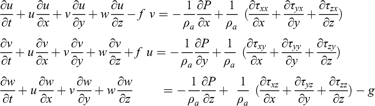 (4.16)
 where the terms τij represent the shear stresses (kg m−1 s−2), which are due to the fluid viscosity. For a newtonian fluid, Newton’s law of viscosity applies. It is written for fluid motion in a single direction as follows:
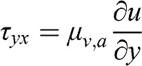 (4.17)
 where μv,a is the dynamic viscosity of the air (kg m−1 s−1). This equation may be seen as the flux in the y direction of the momentum in the x direction. This law, defined for a fluid moving in a given direction (here, x), has been generalized by Navier, Stokes, and Poisson for a fluid moving in three dimensions. Then, the shear stresses for momentum in the x direction are as follows:
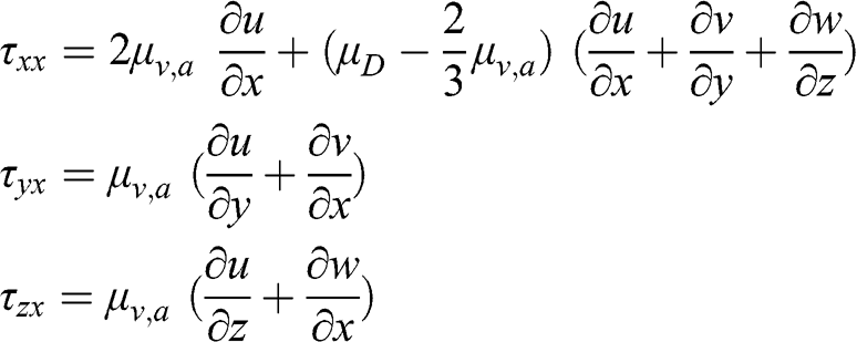 (4.18)
 The other terms for the y and z directions, τxy, τyy, τzy, τxz, τyz, and τzz, are written similarly. Clearly: τxy = τyx, τyz = τzy, and τxz = τzx. In these equations, μv,a is the dynamic viscosity of the fluid and μD is the dilatational viscosity of the fluid (μD = 0 for a monoatomic gas and μD ≈ 0 for air).
Boussinesq introduced several assumptions that apply to the PBL:
– The kinematic viscosity and the molecular thermal conductivity are constant (i.e., their dependence on pressure and temperature can be neglected).
– The heat produced by the viscous forces is negligible compared to solar radiation in the heat transfer equation.
– The atmosphere is considered to be incompressible, since it is an open system (except at the Earth’s surface).
– The fluctuations of the state variables (pressure, temperature, and density) are small compared to their mean values.
– The ratio of the pressure fluctuation and the mean pressure is small compared to the ratio of the temperature fluctuation and the mean temperature and compared to the ratio of the density fluctuation and the mean density.
– The fluctuations of the density are important only when the density is multiplied by the gravitational constant; indeed, the Earth’s surface introduces a constraint on the system in the vertical direction.
The last two assumptions are commonly called the Boussinesq approximation or hypothesis: they imply that the change in the air density can be neglected except in the term (ρa g dz) of the hydrostatic equation (see Equation 3.2).
Using the Boussinesq hypothesis, the continuity equation for momentum is as follows:
 (4.19)
 For u, the friction term may be written as follows (assuming that μv,a is spatially uniform):
 (4.20)
 Changing the order of the derivations:
 (4.21)
 According to the continuity equation, the last two terms are zero. Since the kinematic viscosity, νv,a(m2 s−1), is equal to the ratio of the dynamic viscosity and the fluid density, μv,a/ρa:
 (4.22)
 Thus, the Navier-Stokes equations may be written as follows:
 (4.23)
 where u, v, and w are the wind velocities (m s−1) in the x, y, and z directions, respectively, f is the Coriolis parameter (s−1), ρa is the air density (kg m−3), P is the atmospheric pressure (Pa), νv,a is the kinematic viscosity of the air (m2 s−1), and g is the acceleration due to gravity (m s−2).
The Reynolds number, Re, may be used to estimate whether a flow is turbulent or laminar. It represents the ratio of inertial forces and viscous forces, and it is defined as follows:
 (4.24)
 where u is the velocity of the flow, lc is a characteristic length of the flow, and νv,a is the kinematic viscosity (νv,a = 1.55 × 10⁻⁵ m2 s−1 at 1 atm and 25 °C). For a wind velocity of 10 m s−1 and a characteristic length corresponding to the PBL height, say 1,000 m:
A flow is considered to be turbulent when Re > 3,000. Therefore, the atmospheric flow within the PBL is without any doubt turbulent.
In a turbulent flow, the velocity varies randomly around a mean value. Therefore, it may be written as the sum of a mean value and a term that represents the fluctuation around that mean value (according to the statistical representation of Reynolds):
 (4.25)
 where u¯ represents the mean value of the velocity and u’ represents the random fluctuation around that mean value. The Navier-Stokes equations may then be written as a function of these mean and random terms. Applying the continuity equation for momentum, the Navier-Stokes equations may be rewritten as follows:
 (4.26)
 By decomposing the velocities as the sum of a mean value and a fluctuation around that mean value (Reynolds decomposition), we obtain for u (similar equations may be written for v and w):
 (4.27)
 Averaging over time leads to the Navier-Stokes equation averaged according to the Reynolds decomposition, i.e., RANS for “Reynolds-averaged Navier-Stokes.” Since the mean of the fluctuation term around the mean is by definition zero, the following relationships apply:
 (4.28)
 The RANS equation for u is then as follows:
 (4.29)
 The terms that include the random variables u’, v’, and w’ represent turbulence, and their products are called the Reynolds stresses:
 (4.30)
 Similar terms may be obtained for v and w. Note that these Reynolds stresses, as defined here, have units of m2 s−2 and not the units of a standard stress, which are kg m−1 s−2; the unit of a standard stress would be obtained if the terms on the right-hand sides were multiplied by the fluid density.
There is a set of nine Reynolds stresses, which are called the Reynolds tensor. Because of symmetry between Rxy and Ryx, Rxz and Rzx, and Ryz and Rzy, there are six unknowns in the Navier-Stokes equations, which result from the turbulent nature of the atmospheric flow. New equations must, therefore, be introduced to “close” this system. Several approaches have been proposed to close the RANS equations with an explicit representation of the turbulent terms.
4.3.3 Closure of the Equations of Turbulent Flows
The Boussinesq hypothesis allows one to introduce a relationship between the momentum turbulent term and the mean value of the flow velocity. One introduces the turbulent kinematic viscosity, KM (m2 s−1), which is defined as follows (here for the x and z directions) by analogy with the shear stress (τzx=μv,a∂u∂z)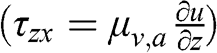 :
:
 (4.31)
 However, note that this analogy is approximate, because the dynamic viscosity, μv,a, is a property of the fluid (here, the air), whereas the turbulent kinematic viscosity is a characteristic of the flow. KM must be defined. Prandtl introduced the concept of a characteristic mixing length, lm, which characterizes the length over which a turbulent eddy will retain its properties before mixing with the surrounding fluid. A dimensional analysis implies that the turbulent kinematic viscosity may be expressed as the product of a characteristic velocity, u* (called the friction velocity), and this characteristic mixing length, lm:
The friction velocity is defined as the square root of the product of the fluctuations of the horizontal and vertical velocities:
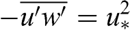 (4.33)
 The friction velocity represents the amplitude of the vertical turbulent flux of the horizontal momentum within the surface layer. Equations 4.31 to 4.33 lead to the following results:
 (4.34)
 The mixing length is not constant, but depends on the distance from the wall (here, the Earth’s surface). This relationship uses the von Kármán constant, κ, taken here to be equal to 0.4:
Therefore, the turbulent kinematic viscosity is expressed as follows:
The friction velocity, u* , is on the order of 0.1 to 0.5 m s−1 for standard atmospheric conditions.
4.3.4 Kinetic Energy of the Atmospheric Flow
The specific kinetic energy of the flow (i.e., kinetic energy per unit mass; m2 s−2) is defined as follows:
 (4.37)
 The mean specific kinetic energy, EkEk , is defined as follows:
 (4.38)
 where kMKE is the specific kinetic energy of the mean flow and kTKE is the mean specific kinetic energy of the turbulent component of the flow (called TKE for ”turbulent kinetic energy”). An equation may be derived for the change in TKE. This equation contains a term, ε, which represents the TKE mean dissipation rate (m2 s−3). Several computational fluid dynamics (CFD) models use the TKE equation to close the RANS equations. Among the models that are the most widely used, one may mention the k-lm, k-ε, and k-ω models (ω is the TKE specific mean dissipation rate). For a more in-depth description of turbulent flow modeling, see, for example, Nieuwstadt et al. (2016).
4.3.5 Vertical Profile of Wind Speed in the Surface Layer
Wind speed changes with height. The vertical profile of wind speed follows a logarithmic law under adiabatic conditions, which results from the assumptions introduced with the first-order closure of turbulence and the use of the Prandtl mixing length (according to Equations 4.34 and 4.35):
 (4.39)
 In the surface layer, the wind speed in a given horizontal direction is given by a differential equation (assuming here for simplicity that the wind direction is in the x direction; i.e., v = 0):
 (4.40)
 For a viscous fluid, the no-slip assumption is generally applied, i.e., the fluid velocity is zero at the surface. However, such a boundary condition does not apply here since the logarithm of zero is not defined and one must introduce a height at which the wind velocity is zero. This height, z0, is called the roughness length. Thus, the wind velocity follows the following profile:
 (4.41)
 The height at which the wind speed becomes zero can be estimated experimentally by extrapolating the wind speed in the vertical direction. Thus, the roughness length can be estimated. This roughness length represents the effect of terrain and obstacles (buildings, vegetation, etc.) on the wind speed vertical profile. As a first approximation, it can be estimated to be in the range of 1/30 to 1/10 of the height of the terrain elements. For example, over grassland with grass about 3 cm high, the roughness length would be in the range of 1 to 3 mm; in an urban area with buildings about 10 m high, the roughness length would be in the range of 30 cm to 1 m.
This logarithmic representation of the vertical wind speed profile is idealized, because no momentum is taken into account below z0. Furthermore, in the case where obstacles affect the atmospheric flow significantly (for example, in a forest or in an urban canopy), a displacement height, db, is introduced, which corresponds to a vertical translation of the surface toward the top of the canopy. For example, for a built area, one may define the displacement height empirically as a function of the fraction of the area that is built, λb, and of the mean building height, hb (MacDonald et al., 1998):
 (4.42)
 For an urban area with a built fraction of, say, 50 % (λb = 0.5), db = 0.75 hb. In the limit, db tends toward 0 as λb tends toward 0 and db tends toward hb as λb tends toward 1.
The vertical profile of the wind speed is then defined above a height (db + z0), at which the wind speed becomes zero. If one wants to represent the flow below that height, one must introduce another model of the atmospheric flow within the canopy. For example, in an urban canopy, experimental data have led to the assumption that the vertical profile of the wind speed may be represented by an exponential function (MacDonald, 2000):
 (4.43)
 where ξb and βb are empirical parameters, which depend on the built area configuration, u(hb) is the wind speed at the top of the canopy (which can be taken to be the wind speed above the canopy multiplied by the cosine of the angle of the wind direction and the street-canyon axis), and hb is the average building height. For example, the following parameterizations may be used (Masson, 2000):

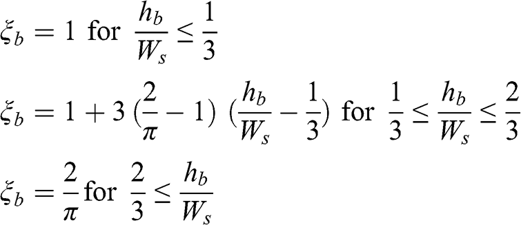 (4.44)
 where Ws is the mean street width. The term hb / Ws is sometimes called the aspect ratio of the street canyon (Landsberg, 1981). Near the street surface, the no-slip condition cannot be satisfied by an exponential profile and a logarithmic profile is used. The vertical profile of the wind speed in an urban area may, therefore, be seen as an ensemble of three connected profiles, which are, starting at the surface:
– a logarithmic profile near the surface
– an exponential profile within the urban canopy
– a logarithmic profile above the urban canopy
These three profiles must connect at heights that are defined by the canopy configuration and atmospheric flow in order to obtain a continuous vertical wind profile (e.g., MacDonald, 2000).
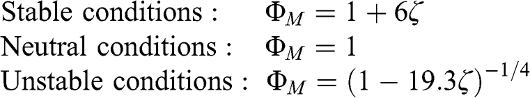
For non-adiabatic conditions, vertical motions are affected by the temperature vertical profile. For neutral adiabatic conditions, one may define the non-dimensional wind shear number, ΦM, as follows:
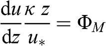 (4.45)
 where by definition, ΦM = 1, according to Equation 4.39. This approach, which involves the use of dimensionless variables (sometimes called “numbers”), has been widely used to define the characteristics of the PBL. Once the standard variables (vertical fluxes, etc.) have been represented using dimensionless functions, the results are applicable regardless of the absolute dimensions. This approach is, therefore, called “similarity theory.” For the PBL, one refers to the similarity theory of Monin-Obukhov (after the names of the two Russian scientists, Andrei Monin and Alexander Obukhov, who proposed it in 1954). This approach has been useful to estimate non-dimensional variables using experimental data for a wide range of atmospheric conditions. Thus, Businger and co-workers (1971) and Dyer (1974) have independently developed corrected vertical profiles for unstable and stable conditions. These profiles use a dimensionless height, ζ. For stable conditions:
For unstable conditions:
These functions were determined experimentally with the assumption that the von Kármán constant was κ = 0.35. For a value κ = 0.4, the following relationships should be used (Jacobson, 2005):
 (4.48)
 In these equations, the dimensionless height, ζ, is defined as (z/LMO), where LMO is the Monin-Obukhov length (as discussed in Section 4.4.3). During daytime, the absolute value of LMO corresponds to the height above which turbulence is generated more by buoyancy (i.e., thermal processes) than by wind shear (i.e., mechanical processes). Its formulation is provided in Equation 4.59. LMO is negative for unstable conditions and is positive for stable conditions. For neutral conditions, LMO is infinite and, therefore, ζ = 0.
The vertical profiles of the wind speed are then obtained by integration:
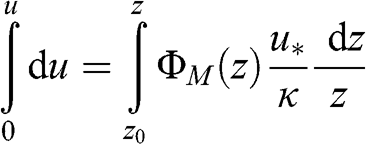 (4.49)
 Analytical solutions may be obtained. For neutral conditions, the solution is straightforward and was provided in Equation 4.41. For stable conditions:
 (4.50)
 where ΦM0 corresponds to the value of ΦM at z = z0. For unstable conditions:
 (4.51)
 For neutral conditions, ζ= 0 and ΦM = 1; therefore, the two profiles represented by Equations 4.50 and 4.51 then become equivalent to the logarithmic profile given by Equation 4.41.
Figure 4.3 depicts vertical profiles of the horizontal wind speed in a surface layer of 100 m depth for stable conditions (Equation 4.50), neutral conditions (Equation 4.41), and unstable conditions (Equation 4.51). The assumptions regarding the roughness length, the friction velocity, and the Monin-Obukhov length are provided in the figure caption. The vertical gradient of the wind speed is much more pronounced when the atmosphere is stratified, and it becomes rapidly negligible above the surface when the conditions are unstable.

Figure 4.3. Vertical profiles of the horizontal wind speed in the surface layer for stable, neutral, and unstable conditions above 1 m. The assumptions are a roughness length (z0) of 0.1 m, a friction velocity (u*) of 0.3, 0.4, and 0.5 m s−1, respectively, and a Monin-Obukhov length (LMO) of 50 m, infinite, and −20 m, respectively.
4.4 Heat Transfer
4.4.1 Heat Transfer Equation
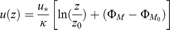
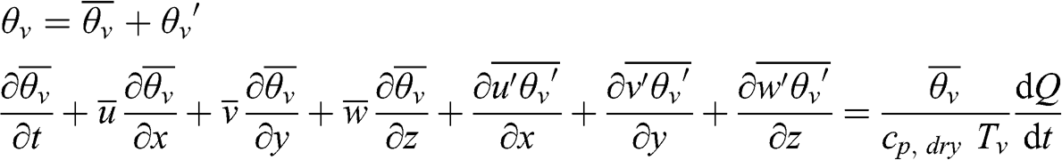
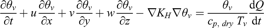
The heat transfer equation may be written as follows, using the virtual potential temperature, θv:
 (4.52)
 where Tv is the virtual temperature (K), Q is the amount of heat exchanged by the system (J kg−1), cp,dry is the specific heat capacity of dry air (J kg−1 K−1), and the term on the right-hand side represents the sources and sinks of heat, i.e., the rates of heat transfer due to changes in water phases (condensation, evaporation, freezing, and melting), solar radiation (absorption of solar radiation in the ultraviolet, visible, and infrared ranges and infrared radiation emission by the Earth’s surface and by greenhouse gases), and human activities (heating, transportation, industrial activities, etc.). This equation may be rewritten as follows:
 (4.53)
 The Boussinesq assumption implies (see Equation 4.19) that the fifth term is zero.
4.4.2 Sensible Heat Flux
Turbulence affects the atmospheric flow, as well as any associated variable. Thus, temperature is a turbulent variable, which can be decomposed following the Reynolds approach using a mean value and a random component around that mean value. The heat transfer equation in its Reynolds average form is written as follows:
 (4.54)
 A first-order closure may be performed using the turbulent heat transfer coefficient, KH (m2 s−1):
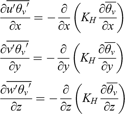 (4.55)
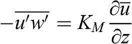
 The last term represents heat transfer via the vertical turbulent flux, which transfers heat from the Earth’s surface toward the atmosphere (see Chapter 5). It is related to the sensible heat flux, which is defined as follows (J m−2 s−1):
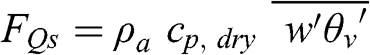 (4.56)
 Then, the heat transfer equation is written as follows (using for simplicity the notation θvθv for θ¯v and u, v, and w for u¯
 , v¯
, v¯ , and w¯
 ):
):
 (4.57)
 4.4.3 Variables Characterizing the PBL Stability
In the surface layer, a temperature scale, θ*, may be introduced, which is related to the sensible heat flux at the surface and which characterizes the production of turbulence via heat transfer:
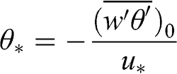 (4.58)
 Using the friction velocity, which characterizes the production of turbulence via mechanical processes (flow affected by terrain and/or obstacles), and the temperature scale, a length scale, LMO, may be defined, which is called the Monin-Obukhov length:
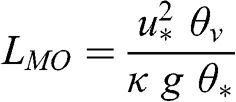 (4.59)
 Thus, the Monin-Obukhov length (Monin and Obukhov, 1954) represents during daytime the height above which the production of turbulence via buoyancy dominates the production of turbulence via mechanical processes (i.e., wind shear). A negative value of LMO implies that the atmosphere is unstable because of heat transfer. A positive value of LMO corresponds to a stable atmosphere. Under neutral conditions, LMO tends to infinity, since the heat flux tends toward zero and, therefore, θ* tends toward zero. The following ranges of LMO are typical of atmospheric conditions: very unstable conditions when LMO ranges between 0 and –10 m, unstable conditions when LMO is less than –10 m, neutral conditions when LMO has very high values (>100 m in absolute value), stable conditions when LMO is greater than 30 m, and very stable conditions when LMO ranges between 0 and 30 m. However, these ranges are rough estimates.
The non-dimensional Richardson numbers are also used to characterize the atmospheric stability (they are named after the English mathematician and physicist Lewis Fry Richardson). The flux Richardson number is expressed as follows:
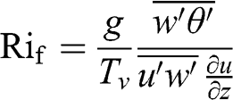 (4.60)
 The gradient Richardson number is expressed as follows:
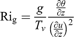 (4.61)
 where Tv is in K. The bulk Richardson number, Rib, is derived from Rig by using discretized vertical gradients of temperature and horizontal wind speed, obtained from meteorological measurements at distinct heights:
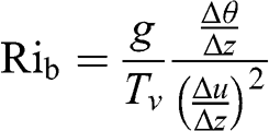 (4.62)
 A positive Richardson number corresponds to a stable atmosphere and a negative Richardson number corresponds to an unstable atmosphere. For a neutral atmosphere, Ri = 0. The Richardson numbers depend on the height at which they are estimated, since the vertical gradients of wind speed and temperature are functions of z. At a given height (or within a given atmospheric layer in the case of Rig and Rib), they represent the ratio of the heat-generated turbulence (represented by the sensible heat flux or the vertical temperature gradient) and mechanically generated turbulence (represented by the friction velocity and/or the vertical gradient of the horizontal wind speed). Therefore, the Richardson number is qualitatively the inverse of the Monin-Obukhov length (in a dimensionless form) and there is a theoretical relationship between Rig (or Rib) and the dimensionless form of the Monin-Obukhov length:
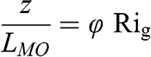 (4.63)
 where z is the height at which Rig (or Rib) is estimated and φ is a dimensionless parameter, which depends on the meteorological conditions; φ is a function of (z / LMO) in the relationship proposed by Monin and Obukhov (1954). For example, according to experiments conducted over the sea, φ may vary between 4 and 21 depending on the temperature gradient and the wind speed (Hsu, 1989). Other relationships between LMO and Rib have been developed based on theoretical considerations and experimental data, in order to estimate LMO from the same measurements as those used to estimate Rib.
The convective velocity, w*, is sometimes used to quantify the intensity of vertical motions within the PBL during unstable conditions:
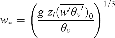 (4.64)
 where g is the acceleration of gravity, zi is the PBL height, θv is the virtual potential temperature, and (w‘θv‘¯)0 represents the sensible heat source at the surface. The convective velocity is on the order of 1 to 2 m s−1 for daytime conditions with strong solar radiation.
For calm atmospheric conditions (u ≈ 0), the friction velocity tends toward zero and, therefore, the Monin-Obukhov length also tends toward zero. Therefore, it is not appropriate as a measure of atmospheric stability if heat-generated convection is important. Under such conditions, one may use the convective temperature scale, θ*C, which is defined with respect to w* (instead of θ*, which is defined with respect to u*, as shown in Equation 4.58), to characterize the importance of the local thermal convection:
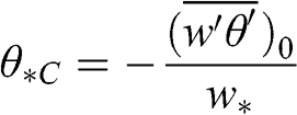 (4.65)
 4.4.4 Vertical Temperature Profiles
The vertical heat flux can be expressed in a dimensionless manner, introducing the variable ΦH, similarly to the vertical momentum flux:
 (4.66)
 where θv is the virtual potential temperature and θ* is the potential temperature scale defined previously. The virtual potential temperature profile is obtained by integrating in the vertical direction:
 (4.67)
 For a neutral atmosphere (i.e., under adiabatic conditions), ΦH = Prt, where Prt is the turbulent Prandtl number. This dimensionless number is defined as the ratio of the turbulent diffusion coefficients for momentum and heat. Businger and coworkers estimated Prt = 0.74 assuming that the von Kármán constant was κ = 0.35. Assuming that κ = 0.4 (i.e., the value most commonly used), then using Prt = 0.95 leads to the same results as those obtained by Businger et al. Similarly to the approach used to obtain the vertical profiles of the horizontal wind speed, empirical values have been developed for ΦH to obtain vertical profiles of the virtual potential temperature under stable and unstable conditions. These profiles are expressed as a function of a dimensionless height, ζ = z/LMO. The functions of ΦH developed by Businger and coworkers used the assumption that κ = 0.35. The functions presented next correspond to κ = 0.4 (Jacobson, 2005).
Under stable conditions:
Under unstable conditions:
Then, the vertical profiles of the virtual potential temperature are as follows. Under neutral conditions:
 (4.70)
 Since there is no sensible heat flux: w‘θ‘¯=0 , therefore, θ* = 0 and θv(z) = θv(z0). Thus, the potential temperature is constant with height under neutral conditions.
Under stable conditions:
 (4.71)
 Under unstable conditions:
 (4.72)
 where ΦH0 corresponds to the value of ΦH at z = z0. The vertical profiles of the virtual potential temperature given by Equations 4.71 and 4.72 tend toward a constant value when the atmospheric conditions become neutral, since the Monin-Obukhov length then tends toward infinity and θ* tends toward zero.
4.4.5 Latent Heat Flux
The latent heat flux corresponds to the water vapor flux associated with evapotranspiration of vegetation and evaporation of water from the surface. This vertical transport of water vapor from the Earth’s surface to the atmosphere results from the heat added to the surface by solar radiation. When the water vapor condenses later in the atmosphere (leading to cloud formation), the condensation process leads to heat production. Therefore, the water vapor flux from the surface to the atmosphere corresponds to a hidden heat flux (the Latin “latens” means hidden).
4.5 Local Circulations: Land-Sea Breezes and Mountain-Valley Winds
The phenomena of land-sea breezes in coastal regions and mountain-valley winds in mountainous regions result from temperature differences at the surface, that lead to differences in air density and, therefore, pressure gradients.
In a coastal region, the land surface has a greater temperature change during the diurnal cycle than the sea surface. This difference is due to the fact that land has a smaller heat capacity (1,350 kJ m−3 K−1 for dry soil) than water (4,200 kJ m−3 K−1); i.e., soil requires less heat than water to increase its temperature by one degree; conversely, a given heat flux will lead to a greater temperature increase on land than at sea. Furthermore, heat transfer occurs in soil only by conduction, whereas heat transfer occurs both by conduction and convection (vertical mixing) in water. Therefore, during the day, solar radiation leads to a greater increase in temperature over land than at sea. As a result, the air layer near the land surface becomes warmer than the air layer near the sea surface. Since warm air is less dense than cold air, the air over land will rise, leading to a decrease in pressure. The pressure gradient corresponds to greater pressure over the sea than over land and it leads to a wind coming from the sea toward the land, i.e., a sea breeze. This air circulation at the surface is then completed aloft by a returning flow from the land toward the sea.
At night, the land surface releases the heat absorbed during the day back to the atmosphere via infrared radiation (see Chapter 5). Thus, the land surface temperature decreases faster than that of the sea surface. Then, a land breeze sets up at night, which is in the opposite direction of the daytime sea breeze. The temperature difference is generally less at night than during the day. Therefore, a land breeze is generally weaker than the corresponding sea breeze. Figure 4.4 depicts these land-sea breeze processes.
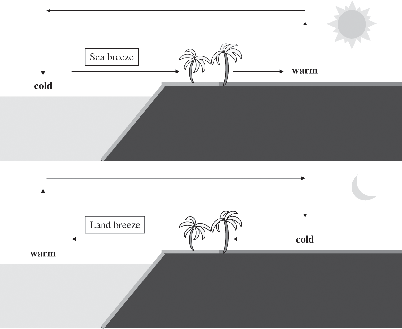
Figure 4.4. Schematic representation of sea and land breezes. Top figure: daytime sea breeze; bottom figure: nighttime land breeze. The terms “warm” and “cold” are relative to one another and characterize the temperature gradient.
In a mountainous region, the hills and snowless mountain tops warm up more during the day than the valleys, because the former have better exposure to solar radiation. As a result, a phenomenon similar to that of the land-sea breeze takes place. During the day, the air near the mountain top becomes warmer than that of the valleys. There is, therefore, a slight decrease in the atmospheric pressure near the mountain top compared to the valley and the atmospheric flow at the surface will be from the valley toward the mountain top. This is the valley breeze. The atmospheric local circulation is completed by a reverse atmospheric flow aloft. At night, the infrared radiation from the surface is more efficient at the mountain top, which cools down faster than the valley. Therefore, a mountain breeze sets up from the mountain top toward the valley. If the flow occurs along the axis of a valley, a similar phenomenon will occur between the upper and lower parts of the valley. Figure 4.5 depicts these mountain-valley breeze processes.
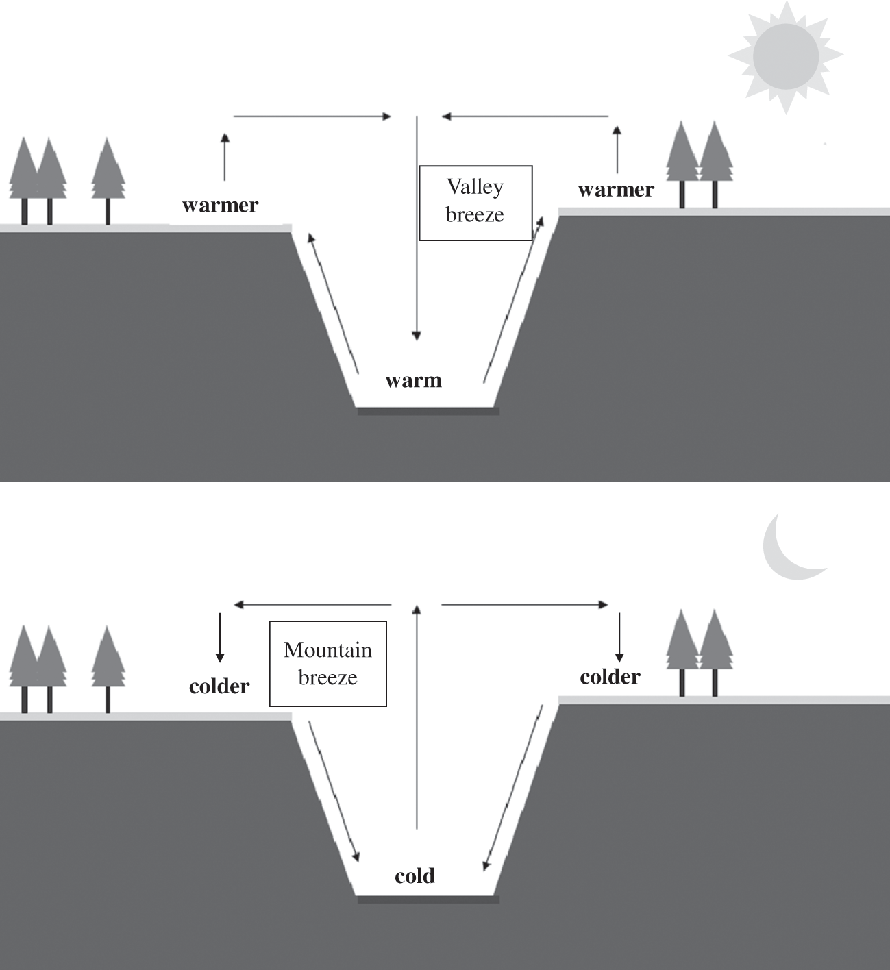
Figure 4.5. Schematic representation of the mountain and valley breezes. Top figure: daytime valley breeze; bottom figure: nighttime mountain breeze. The terms “warm” and “cold” reflect the daytime and nighttime conditions, respectively.
4.6 Meteorological Modeling
Numerical modeling of the atmospheric flows is performed using meteorological models. The equations that must be solved numerically include the Reynolds-averaged Navier-Stokes (RANS) equations, the heat transfer equation, radiative transfer through the atmosphere (see Chapter 5), and mass conservation for water. The equations for the atmospheric flows are by nature chaotic, i.e., the solution is very sensitive to the initial conditions (Lorenz, 1963). This chaotic behavior is the main reason why meteorological forecasts degrade after a few days. Currently, the Weather Research & Forecasting model (WRF; www.wrf-model.org/) is the main numerical model being used to generate three-dimensional (3D) fields of pressure, temperature, humidity, winds, and turbulence, as input data for air quality models. For air quality studies pertaining to past periods, it is possible to obtain 3D meteorological fields from organizations such as the United States National Centers for Environmental Prediction (NCEP; www.ncep.noaa.gov/) and the European Centre for Medium-Range Weather Forecasts (ECMWF; www.ecmwf.int/). These fields are re-analyses, i.e., meteorological data have been assimilated into the numerical model to obtain an optimal representation of the meteorological fields (Kalnay, 2003). Descriptions of the processes and equations of meteorological models are available, for example, in the books by Pielke (2013) and Jacobson (2005).
Problems
Problem 4.1 Potential temperature and atmospheric stability
The temperature is 20 °C at sea level and 16 °C at an altitude of 500 m. The atmosphere is assumed to be dry.
a. Calculate the potential temperature at 500 m.
b. Is the atmosphere stable, neutral, or unstable?
Problem 4.2 Reynolds number and atmospheric turbulence
a. Calculate the Reynolds number in the atmospheric planetary boundary layer (PBL) under the following conditions: a low wind speed of 2 m s−1, a wintertime PBL height of 500 m, and a kinematic viscosity of the air of 1.55 × 10⁻⁵ m2 s−1.
b. Is this value of the Reynolds number characteristic of a turbulent or laminar regime?
Problem 4.3 Friction velocity and roughness length
The following measurements of wind speed as a function of height are available:
| Altitude (m) | Wind speed (m s−1) |
|---|---|
| 0.25 | 3.76 |
| 0.5 | 4.62 |
| 1 | 5.31 |
| 2 | 6.11 |
| 4 | 6.75 |
| 8 | 7.72 |
| 16 | 8.59 |
Calculate the roughness length, z0, and the friction velocity, u*, corresponding to these experimental data, assuming that the atmosphere is neutral.
Problem 4.4 Land-sea breezes
In a coastal region where land-sea breezes occur, a freeway is located along the seashore. A residential area is located inland a few hundred meters from the freeway. Will this residential area be affected by the freeway traffic emissions during the day or at night?