Abstract
Symmetric Archimedean copulas are widely applied for hydrologic analyses for the following reasons: (1) they can be easily constructed with the given generating function; (2) a large variety of copulas belong to this class (Nelsen, 2006); and (3) the Archimedean copulas have nice properties, such as simple and elegant mathematical treatment. This chapter focuses on the symmetric Archimedean copulas.
4.1 Definition of Symmetric Archimedean Copulas
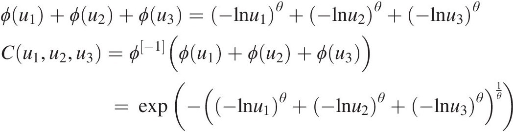
Formally, a d-dimensional Archimedean symmetric copula Cd : [0, 1]d→[0, 1]Cd:01d→01 can be defined as follows (Nelsen, 2006; Salvadori et al, 2007; Savu and Trede, 2008). We first show it for a two-dimensional case and how it is constructed:
 (4.1)
(4.1)In Equation (4.1), ui, i = 1, 2,…,d, the marginal cumulative distribution function (CDF) of the ith random variable; and ϕ(⋅)ϕ⋅ is the generating function of the Archimedean copula, which has the following properties:
ϕ(⋅)ϕ⋅ is a continuous strictly decreasing function from [0, 1]→[0, ∞)01→0∞, we have ϕ(1) = 0ϕ1=0 and ϕ(0) = ∞ϕ0=∞, i.e., for ϕ(uk), k = 1, …, d; uk ∈ [0, 1], ϕ(uk) ∈ [0, ∞)ϕuk,k=1,…,d;uk∈01,ϕuk∈0∞.
ϕ[−1]ϕ−1 is the pseudo-inverse function of ϕϕ and nonincreasing on [0, ∞)0∞. ϕ[−1]ϕ−1 is strictly decreasing on [0, ϕ(0)]0ϕ0 with Domϕ[−1] ∈ [0, ∞)Domϕ−1∈0∞ and Ranϕ[−1] ∈ [0, 1]Ranϕ−1∈01 as follows:
ϕ−1=ϕ−1t;0≤t≤ϕ00;ϕ0≤t<∞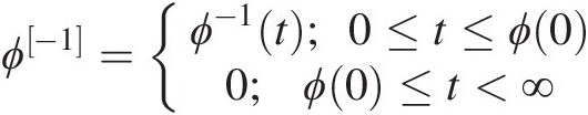 (4.2)
(4.2)
ϕ[−1]ϕ−1 also has derivatives of all orders which alternate in sign, i.e., for all t to be in [0, ∞)0∞.
With k = 0, 1, …,k=0,1,…, it satisfies the following:
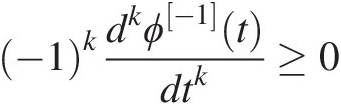 (4.3)
(4.3)Following Equation (4.1), the two- and three-dimensional symmetric Archimedean copulas can be written as follows:
It should be noted that as the name of symmetric Archimedean copulas suggests, there is the same degree of dependence among all possible pairs for d ≥ 3d≥3. This fact usually hinders the application of symmetric Archimedean copulas for multivariate analysis in higher dimensions, since the dependence among the possible pairs in reality is usually not the same. We will illustrate it in subsequent chapters.
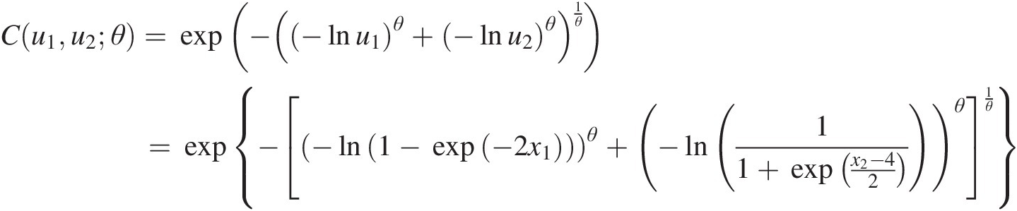
Example 4.1 Show that the function ϕ(t) = (− ln t)θ, θ ≥ 1ϕt=−lntθ,θ≥1 is the generating function of Archimedean copula, and express the corresponding two- and three-dimensional copulas with this generating function.
Solution: To show ϕ(t) = (− ln t)θ, θ ≥ 1ϕt=−lntθ,θ≥1 is the generating function of Archimedean copulas, we need to show that it is a continuous strict decreasing function.
1. Let f(t) = ln tft=lnt. It is obvious that f(t)ft is a strictly increasing function of t and thus −f(t) = − ln t−ft=−lnt is a strict decreasing function of t with − ln (0)→ ∞ , − ln (1) = 0.−ln0→∞,−ln1=0. Given θ ≥ 1θ≥1, we have (− ln (0))θ = ∞θ = ∞ ; (− ln (1))θ = 0∞ = 0−ln0θ=∞θ=∞;−ln1θ=0∞=0. Now we show ϕ(t) = (− ln t)θ, θ ≥ 1ϕt=−lntθ,θ≥1 satisfies the generating function ϕ(t) = (− ln t)θ, θ ≥ 1ϕt=−lntθ,θ≥1 is a continuous strictly decreasing from [0, 1]→[0, ∞)01→0∞.
2. The inverse of function ϕ(t)ϕt can be given as follows:
Let u = (− ln t)θ.u=−lntθ. Then we have ϕ−1t=exp(−u1θ)
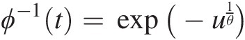 . Now we need to show that ϕ−1(t)ϕ−1t is nonincreasing. And, it is obvious that the exponential function above is continuous and a nonincreasing function.
Applying Equation (4.1) for d = 2 or 3, we have the following:
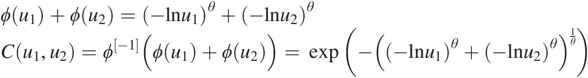 (4.6a)
and
 (4.6b)
To illustrate the copula with the random variables in a real domain, let random variables {X1, X2, X3}X1X2X3 be positively dependent, and they may be modeled with the symmetric Archimedean copula in Equation (4.6b). In addition, X1, X2, X3X1,X2,X3 follow the marginal distributions, respectively, of
We then have u1=F1x1=1−exp−2×1,u2=F2x2=11+exp−x2−42,u3=Φx3−32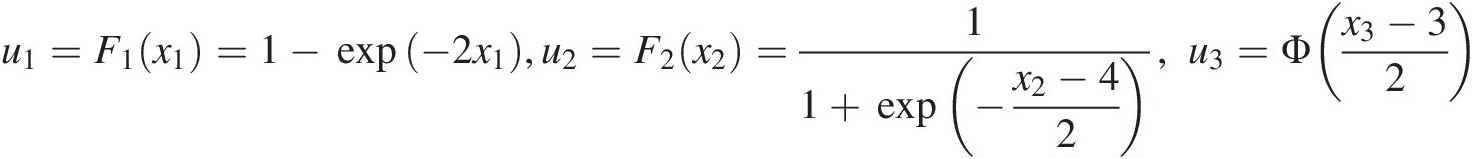 . Now we have the following copula functions:
 (4.7a)
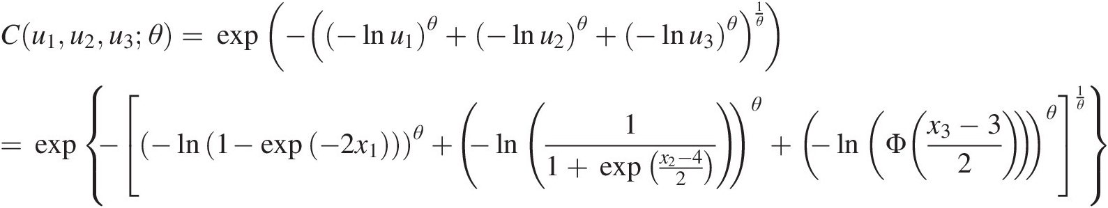 (4.7b)
Equations (4.7a) and (4.7b) illustrate how to construct symmetric Archimedean copulas from the correlated random variables with following different marginal distributions. It may be worth noting here again that all cumulative marginal distribution ui~uniform (0, 1)ui~uniform01.
4.2 Properties of Symmetric Archimedean Copulas
Let C be an Archimedean copula with generating function ϕϕ. The Archimedean copula has the following properties (Nelsen, 2006; Salvadori et al., 2007; Savu and Trede, 2008):
C is permutation-symmetric in its d arguments. This indicates that the Archimedean copula is the distribution function of d exchangeable uniform random variates.
C is associative.
If α>0α>0 is any constant, then αϕαϕ is also a generator of C.
Example 4.2 Show for a given bivariate Archimedean copula function, one has C(u1, u2) = C(u2, u1)Cu1u2=Cu2u1.
Solution: Directly from Equation (4.1),
Example 4.3 Show that the copula is associative.
Suppose the symmetric Gumbel–Hougaard copula with parameter θ can be applied to study a given trivariate analysis. Show that the copula is associative, as follows:
Solution: The trivariate symmetric Gumbel–Hougaard copula can be expressed as follows:

in which ϕ(u) = (− ln u)θϕu=−lnuθ.
Now let’s prove the associative property of the symmetric copula using C(u1, C(u2, u3))Cu1Cu2u3 as an example. The inner copula function C(u2, u3)Cu2u3 is the bivariate Gumbel–Hougaard copula with the same parameter θ and can be written as follows:

Then C(u1, C(u2, u3))Cu1Cu2u3 is also the bivariate Gumbel–Hougaard copula and can be written as follows:

Finally, we have the following:

Similarly, we can prove that C(u1, u2, u3) = C(C(u1, u2), u3).Cu1u2u3=CCu1u2u3.
Equation (4.9) implies that given three random variables u1, u2, u3,u1,u2,u3, the dependence between the first two random variables taken together and the third one alone is the same as the dependence between the first random variable taken alone and the two last ones taken together. This implies a strong symmetry between different variables in that they are exchangeable (Malevergne and Sornette, 2006). But the associative property of the Archimedean copula is not satisfied by other copula families in general (Embrechts et al., 2001).
Example 4.4 Given the information u=12,v=14,w=16,andθ=12 , show that the associative property cannot be applied to the Farlie–Gumbel–Morgenstern copula.

Solution: The bivariate Farlie–Gumbel–Morgenstern copula can be expressed as follows:
With u=12,v=14,w=16,andθ=12 , we have


and


Now we can reach the conclusion: C(u1, C(u2, u3))≠C(C(u1, u2), u3).Cu1Cu2u3≠CCu1u2u3.
Example 4.5 Using the bivariate Gumbel–Hougaard copula, show αϕαϕ is also a generator.
Solution: The generating function and the corresponding Gumbel–Hougaard copula can be written as follows:


in which θθ is the copula parameter.
For any given α, α>0α,α>0 and let ψ(t) = αϕ(t) = α(− ln t)θψt=αϕt=α−lntθ, we have the following:

Rearranging the preceding Gumbel–Hougaard copula function, we have the following:
 (4.10)
Now, we show that αϕαϕ is also a generator of the Archimedean copula C, if α>0α>0.
Let U1, …, UdU1,…,Ud be d (dimensional) random variables with the joint distribution represented by the Archimedean copula C and generator ϕϕ. The distribution function of C(U1, …, Ud)CU1…Ud, i.e., Kendall distribution, KCKC, can be expressed as follows:
KCt=PCU1…Ud≤t=t+∑i=1d−1−1iϕiti!fi−1t (4.11)

where the auxiliary functions f0=1ϕ’t , and fi(t)fit for i ≥ 1i≥1 are defined recursively as fit=fi−1’tϕ’t
 . For bivariate case, KCt=t−ϕtϕ’t
 . An Archimedean copula is determined by the function KC(t)KCt defined on the unit interval [0,1]. This is a very useful result to determine which parametric copula family fits the data best (Savu and Trede, 2008).
From Section 3.4.2, we can derive the expression between Kendall’s τnτn and parameter of symmetric Archimedean copulas using K(t)Kt. Let bivariate random variables X and Y be modeled by the Archimedean copula, u = FX(x), v = FY(y).u=FXx,v=FYy. Then for the bivariate Archimedean copula C(u, v)Cuv, Equation (3.73) can be rewritten as follows:
 (4.12)
Example 4.6 Consider the Gumbel–Hougaard copula with generator ϕ(t) = (− ln t)θ, θ ≥ 1ϕt=−lntθ,θ≥1. Derive Kendall’s τ from the Gumbel–Hougaard copula.
Solution: Taking the first derivative of ϕ(t)ϕt,ϕ’t=−θ−lntθ−1t,ϕtϕ’t=−lntθ−θ−lntθ−1t=tlntθ ; Kendall’s ττ for the Gumbel–Hougaard copula is as follows:
 (4.13)
Furthermore, in Equation (4.13) τ = 0τ=0 if θ = 1θ=1 (i.e., the bivariate random variable is independent), and the dependence increases with the increase of copula parameter θθ.
Example 4.7 Consider the Clayton copula with generator ϕt=t−θ−1θ and parameter θ : θ ∈ [−1, ∞)\0θ:θ∈−1∞\0. Derive Kendall’s τ from the Clayton copula.

Solution: Taking the first derivative of ϕ(t)ϕt, we have the following:

Kendall’s ττ for the Clayton copula can then be computed as follows:
 (4.14)
In Equation (4.14), τ = − 1τ=−1 when θ = − 1θ=−1 (i.e., perfectly negatively dependent). And τ→1τ→1 when θ→∞θ→∞ (i.e., perfectly positively dependent). Similar to Example 4.6, the dependence of the bivariate random variable increases with the increase of parameter θθ.
4.3 Archimedean Copula Families
4.3.1 Bivariate Archimedean Copula Families
There exists a large variety of symmetric Archimedean copula families that are used for constructing copulas to represent multivariate distributions. Table 4.1 lists the popularly applied one-parameter Archimedean copulas (Nelsen, 2006). Tables 4.2 and 4.3 list their first-order derivative of ∂∂u1Cu1u2 and the copula density c(u1, u2)cu1u2, respectively. One may refer to Nelsen (2006) for other one-parameter Archimedean copulas.
Table 4.1. Selected Archimedean copulas.
| Name | Copula function Cθ(u1, u2)Cθu1u2 | Generating function ϕ(t)ϕt | Parameter θθ |
|---|---|---|---|
| Clayton | maxu1−θ+u2−θ−1−1θ0 | 1θt−θ−1 | [−1, ∞)\{0}−1∞\0 |
| Ali–Mikhail–Haq | u1u21+1−u1θ1−u2θ1θ | ln1−θ1−tt | [−1, 1]−11 |
| Gumbel–Hougaard | exp−−lnu1θ+−lnu2θ1θ | (− ln t)θ−lntθ | [1, ∞)1∞ |
| Frank | −1θln1+e−θu1−1e−θu2−1e−θ−1 | −lne−θt−1e−θ−1 | (−∞, ∞)\{0}−∞∞\0 |
| Joe | 1−1−u1θ+1−u2θ−1−u1θ1−u2θ1θ | − ln (1 − (1 − t)θ)−ln1−1−tθ | [1, ∞)1∞ |
| Survival | u1u2e−θ ln u1 ln u2u1u2e−θlnu1lnu2 | ln(1 − θ ln t)ln1−θlnt | (0, 1]01 |
Table 4.2. First-order derivatives ∂∂u1Cθu1u2 for the selected Archimedean copulas.

| Name | ∂∂u1Cθu1u2 |
|---|---|
| Clayton | u1−1−θ−1+u1−θ+u2−θ1+θθ,θ>0 |
| Ali–Mikhail–Haq | u2+θu2−1+u2−1+θ−1+u1−1+u22 |
| Gumbel–Hougaard | −lnu1−1+θ−lnu1θ+−lnu2θ−1+1θu1e−lnu1θ+−lnu2θ1θ |
| Frank | e−θu1e−θu2−1e−θu1+u2−e−θu1−e−θu2+e−θ |
| Joe | −1−u1−1+θ−1+1−u2θ1−u1θ+1−u2θ−1−u1θ1−u2θ−1+1θ |
| Survival | u2−θu2lnu2eθlnu1lnu2 |
Table 4.3. Copula density cθ(u1, u2)cθu1u2 for the selected Archimedean copulas.
∂2∂u1∂u2Cθu1u2 | |
| Clayton | |
1+θu1−1−θu2−1−θ−1+u1−θ+u2−θ1+2θθ,θ>0 | |
| Ali–Mikhail–Haq | |
−1+θ2−1+u2+u2−u1u2−θ−2+u1+u2−u1u2−1+θ−1+u1−1+u23 | |
| Gumbel–Hougaard | |
−lnu2−1+θ−lnu1−1+θw2−2θθ−1−θw1−2θθu1u2ew1θ,w=−lnu1θ+−lnu2θ | |
| Frank | |
θeθ−1eθ1+u1+u2eθu1+u2−eθ1+u1−eθ1+u2+eθ2 | |
| Joe | |
1−u11−u2−1+θθ−1+ww1θ−2 w = (1 − u1)θ − ((1 − u1)(1 − u2))θ + (1 − u2)θw=1−u1θ−1−u11−u2θ+1−u2θ w = (1 − u1)θ − ((1 − u1)(1 − u2))θ + (1 − u2)θw=1−u1θ−1−u11−u2θ+1−u2θ | |
| Survival | |
1−θ−θlnu2+θlnu1−1+θlnu2eθlnu1lnu2 |
As discussed in Nelsen (2006), the Cook–Johnson (Clayton) family was derived by Clayton (1978), Oakes (1982, 1986), Cox and Oakes (1984), and Cook and Johnson (1981). This copula family can be used for modeling nonelliptically symmetric (nonnormal) multivariate data (Cook and Johnson, 1981). When θ = − 1θ=−1, the copula represents the joint distribution of the perfectly negatively dependent bivariate random variables, i.e., the Fréchet–Hoeffding lower bound: W : W = max (u1 + u2 − 1, 0)W:W=maxu1+u2−10. When θ = 0θ=0, the copula represents the joint distribution for independent bivariate random variables, i.e., product copula: Π : Π = u1u2Π:Π=u1u2. When θ→∞θ→∞, the copula represents the joint distribution for perfectly positively dependent bivariate random variables, i.e., the Fréchet–Hoeffding upper bound: M : M = min (u1, u2)M:M=minu1u2.
The Gumbel–Hougaard Archimedean copula was first introduced by Gumbel (1960). This copula family cannot be applied to model the negatively dependent bivariate random variables. Nelsen (2006) showed that the Gumbel–Hougaard copula belonged to the extreme value copula family. With this characteristic, the Gumbel–Hougaard Archimedean copula may be a suitable candidate for multivariate frequency analysis of extreme hydrological events, i.e., peak discharge and corresponding volume and duration.
The Ali–Mikhail–Haq Archimedean copula was developed by Ali et al. (1978). It was developed based on the concept of univariate logistic distribution that may be specified by considering a suitable form for the odds in favor of a failure against survival. The parameter of this copula is a measure of departure from independence or a measure of association between two random variables. In addition, the Ali–Mikhail–Haq copula can only capture the dependence within the range of τ ∈ [−0.182, 0.333]τ∈−0.1820.333, which limits the application of the Ali–Mikhail–Haq copula to bivariate frequency analysis.
The Frank Archimedean copula was developed by Frank (1979). The Frank copula satisfies all the conditions for the construction of bivariate distributions with fixed marginals except for independent variables (θ≠0)θ≠0), for the Frank copula). However, if the bivariate random variables are independent, the copula function is the product copula. Thus, the Frank copula is also considered absolutely continuous with full support on the unit square as the Cook–Johnson (Clayton) copula family.
The Joe Archimedean copula was first introduced by Joe (1993). When θ = 1θ=1, this copula represents the joint distribution for independent bivariate random variables. Similar to the Gumbel–Hougaard copula, the Joe copula cannot be applied to model negatively dependent bivariate random variables.
The survival copula is associated with Gumbel’s bivariate exponential distribution. This family is the survival copula that is actually the survival probability distribution of the Gumbel bivariate exponential distribution.
Example 4.8 Using the copulas given in Table 4.4, plot the density functions of bivariate Archimedean copulas. Can any conclusions be reached from these plots?
Table 4.4. Bivariate Archimedean copula parameters.
| Copula | Parameter θθ | |
|---|---|---|
| Clayton | 0.5 | 2 |
| Gumbel–Houggard | 2 | 5 |
| Frank | –5 | 2 |
| Joe | 2 | 5 |
Solution: With the corresponding copula density function listed in Table 4.3, Figure 4.1 plots the copula density functions for the copulas listed in Table 4.4. In the case of the Clayton copula, when θ ∈ [−1, 0)θ∈−10, its generating function is not strict. Thus, the Clayton copula is only sufficiently differentiable if θ>0θ>0. In addition, from Figure 4.1 and the discussion on tail dependence in Chapter 3, we can reach the following conclusions graphically: (1) the random variables are positively dependent and seem to have left (lower) tail dependence but no right (upper) tail dependence for the Clayton copula; (2) the random variables are positively dependent for the Gumbel–Hougaard and Joe copulas and exhibit the right (upper) tail dependence; and (3) the Frank copula does not seem to have either right (upper) or left (lower) tail dependence, and the random variables are negatively dependent when θ < 0θ<0.

Figure 4.1 Copula density plots.
4.3.2 Relation of Kendall’s τ and Parameter θ for Bivariate Archimedean Copulas
Equation (4.9) presents the relation between Kendall’s τ and the generating function of bivariate Archimedean copulas. In turn, the relation between Kendall’s τ and parameter θ for a given bivariate Archimedean copula can be determined. Table 4.5 lists this relation for the selected Archimedean copulas.
Table 4.5. Relations between ττ and θθ for selected symmetric Archimedean copulas.
| Family | ϕ(t)ϕt | ϕ‘(t)ϕ′t | τ=1+4∫01ϕtϕ’tdt | Range of ττ |
|---|---|---|---|---|
| Clayton | 1θt−θ−1 | −t−1 − θ−t−1−θ | θθ+2 | [−1, 1]\0−11\0 |
| Ali–Mikhail–Haq | ln1−θ1−tt | θ−1t−θt+θt2 | No analytical solution | −0.1813 |
| Gumbel–Hougaard | (− ln t)θ−lntθ | −θt−lntθ−1 | 1−1θ | [0, 1]01 |
| Frank | −lne−θt−1e−θ−1 | θ1−eθt | 1−4θD1−θ−1, D1θ=1θ∫00tet−1dt, D1θ=1θ∫00tet−1dt, D1−θ=D1θ+12 D1−θ=D1θ+12 | [−1, 1]\0−11\0 |
| Joe | − ln [1 − (1 − t)θ]−ln1−1−tθ | θ1−tθ−1−1+1−tθ | No analytical solution | [0, 1] |
| Survival | ln(1 − θ ln t)ln1−θlnt | θtlnt−1 | No analytical solution | [−0.3613, 0] |
4.4 Symmetric Multivariate Archimedean Copulas (d ≥ 3d≥3)
Nelsen (2006) stated that the bivariate Archimedean copula may not be extended to a multivariate case, unless additional conditions are satisfied to construct the symmetric multivariate Archimedean copulas to represent the joint distribution of multivariate random variables (i.e., d ≥ 3d≥3). Nelsen (2006) discussed the theorem and three additional useful results that are necessary to construct the appropriate multivariate Archimedean copula. These results are introduced in the following.
Theorem (Theorem 4.6.2, Nelsen, 2006): Let ϕϕ be a continuous strictly decreasing function from I to [0, ∞)0∞ with ϕ(0) = ∞ , ϕ(1) = 0ϕ0=∞,ϕ1=0, and ϕ−1ϕ−1 denote the inverse of ϕϕ. If Cd is the function from Id to I, given by Equation (4.1), then Cd is the copula function to represent the d-dimensional multivariate distribution if and only if ϕϕ is completely monotonic on [0, ∞)0∞, as follows:
 (4.15)
Result 1: If function f is absolutely monotonic, i.e.,
dkf(x)/dxk ≥ 0, k = 0, 1, 2, …dkfx/dxk≥0,k=0,1,2,…(4.16)
and function g is completely monotonic, then the composite f ∘ gf∘g is completely monotonic.
Result 2: If functions f and g are completely monotonic, then so is their product fg.
Result 3: If f is completely monotonic and g is a positive function with a completely monotone derivative, then the composite f ∘ gf∘g is completely monotonic.
Table 4.6 lists the applicability to extend the selected bivariate Archimedean copula to higher dimension.
Table 4.6. Multivariate (d ≥ 3d≥3) symmetric Archimedean copulas.


Example 4.9 Show that the bivariate Clayton copula can be extended to higher dimension symmetric Clayton copulas for θ>0θ>0.
Solution: It is known that if the Clayton copula can be extended to higher dimensions, i.e., d ≥ 3d≥3, we need to satisfy the theorem (Theorem 4.6.2, Nelsen, 2006) discussed previously. The generating function for the Clayton copula can be written as follows:

According to Nelsen (2006), we know that for θ ≥ 0θ≥0, the generating function is strictly decreasing from I to (0, ∞)0∞. Applying Equation (4.15), we have the following:


…

Now, we reach the conclusion that the bivariate Clayton copula can be extended to multivariate symmetric Clayton copula, as follows:

Note that the multivariate symmetric Clayton copula (i.e., d ≥ 3d≥3) may only model the positive dependent/independent multivariate random variables. The reason is that if θ < 0θ<0, Equation (4.15) cannot be guaranteed to be fully satisfied.
Example 4.10 Show that the inverse of the generating function of the Ali–Mikhail–Haq copula is completely monotonic and thus the bivariate Ali–Mikhail–Haq copula can be extended to higher dimensions.
Solution: Following Nelsen (2006), it is known that the generating function of the Ali–Mikhail–Haq copula is strictly decreasing from I to (0, ∞)0∞. The generating function and its inverse function can be written as follows:

Rather than directly applying the theorem as in Example 4.9, here we use the inequality proposed by Widder (1941) for function ϕ−1ϕ−1 to be completely monotonic, as follows:
The first and second derivative of the inverse function can be written as follows:

Substituting the first and second derivatives of the inverse function into Equation (4.17), we have the following:

Considering the Ali–Mikhail–Haq copula with θ ∈ [−1, 1)θ∈−11, we have ϕ−1(ϕ−1)” − ((ϕ−1)‘)2 ≥ 0ϕ−1ϕ−1′′−ϕ−1′2≥0 for the whole parameter range. Finally, we show that ϕ−1ϕ−1 is completely monotonic in t ∈ (0, ∞)t∈0∞ with θ ∈ [−1, 1)θ∈−11. The bivariate Ali–Mikhail–Haq copula can be extended to higher dimensions as follows:

Example 4.11 Show that the Joe copula can be extended to any dimension d ≥ 3d≥3, for θ ∈ [1, ∞)θ∈1∞.
Solution: We will solve this example using the result 1 introduced earlier, that is, for two given functions f and g, if f is absolutely monotonic and g is completely monotonic, then f ∘ gf∘g is completely monotonic.
The generating function and its inverse function of the Joe copula can be written as follows:

To use two previously stated properties stated, we let fx=1−1−x1θ,x∈01 and g(t) = exp (−t)gt=exp−t.
For function f(x)fx, applying Equation (4.11) we have the following:


…

Thus, we know the function f(x)fx is absolutely monotonic.
For function g(t)gt, g(t) = exp (−t) ≥ 0gt=exp−t≥0, we also need to show that g(t)gt is completely monotonic.
The first and second derivatives of function g(t)gt are as follows:
We can also substitute function g(t)gt into Equation (4.15) and have the following:


Now, we have f ∘ gf∘g as completely monotonic. The bivariate Joe copula can be extended to higher dimensions as follows:

4.5 Identification of Symmetric Archimedean Copulas
The Archimedean copulas can be identified using nonparametric, semiparametric, and parametric estimation procedures.
4.5.1 Nonparametric Estimation Procedure for Bivariate Copulas
Genest and Rivest (1993) described a procedure to identify a copula function based on nonparametric estimation for bivariate Archimedean copulas. It is assumed that a random sample of bivariate observations (x11, x21), (x12, x22), …, (x1n, x2n)x11x21,x12x22,…,x1nx2n is available and that its underlying distribution function F(x1, x2)Fx1x2 has an associated Archimedean copula C, i.e., C(FX1(x1), FX2(x2)) = F(x1, x2)CFX1x1FX2x2=Fx1x2. Then, the following steps can be followed to identify an appropriate copula:
1. Determine Kendall’s ττ(the dependence structure of the bivariate random variables) from observations using Equation (3.73).
2. Determine the copula parameter θθ from the preceding value of τ according to the relation between Kendall’s τ and the copula parameter θθ (See Table 4.5), i.e., for the Gumbel–Hougaard copula family, the relation between Kendall’s τ and the copula parameter θθ is given as τn = 1 − 1/θτn=1−1/θ.
3. Obtain the generating function of the copula, ϕϕ, by inserting parameter θθ obtained as in step 2.
4. Obtain the copula from its generating function ϕϕ.
Thus, copula functions based on different bivariate Archimedean copula families are obtained.
Now the identified copula needs to be tested, if it is adequate for given bivariate observations. This is accomplished using the following steps:
1. Define an intermediate random variable Z = F(x1, x2)Z=Fx1x2, which has a distribution function K(z) = P(Z ≤ z)Kz=PZ≤z. This distribution is related to the generator of the Archimedean copula through Equation (4.18).
2. Construct a nonparametric estimate of Kn as follows:
a. Compute the following:
zi=∑j=1n1x1j≤x1iandx2j≤x2in−1,i=1,…,n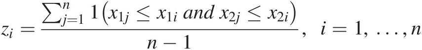 (4.18)
b. Construct nonparametric Kendall distribution (Kn):
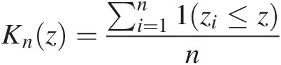
Knt=∑i=1nzi≤tni.e.zi′s≤z. (4.19)
3. Construct a parametric estimate Kendall distribution (K) as follows:
Kt=t−ϕtϕ’t (4.20)


Construct a plot of nonparametric Kn(t)Knt versus parametrically estimated K using Equation (4.20), which may also be called a Q-Q plot. If the plot is in agreement with a straight line passing through the origin at a 45 degree angle, then the generating function is satisfactory. The 45 degree angle indicates that the quantiles are equal. Otherwise, the copula function needs to be reidentified.
Example 4.12 Using the bivariate sample data given in Table 4.7, (1) estimate the parameters if the Gumbel–Hougaard, Frank, and Clayton copulas are tested; (2) construct the Q-Q plot (i.e., nonparametric and parametric Kendall distribution), the K-plot and chi-square plot for each copula candidate; and (3) determine what can be concluded from the plots.
Table 4.7. Sample data: X and Y following gamma and normal distributions, respectively.
| No. | X | Y | No. | X | Y |
|---|---|---|---|---|---|
| 1 | 11.68 | 7.67 | 51 | 12.82 | 6.28 |
| 2 | 18.01 | 15.54 | 52 | 7.79 | 7.49 |
| 3 | 9.15 | 3.03 | 53 | 16.02 | 13.94 |
| 4 | 16.56 | 12.49 | 54 | 14.03 | 12.99 |
| 5 | 7.80 | 7.41 | 55 | 8.53 | 8.46 |
| 6 | 13.11 | 6.36 | 56 | 10.45 | 9.44 |
| 7 | 9.81 | 8.03 | 57 | 18.71 | 13.97 |
| 8 | 11.76 | 11.63 | 58 | 13.60 | 10.89 |
| 9 | 20.59 | 16.60 | 59 | 9.02 | 15.45 |
| 10 | 21.60 | 16.00 | 60 | 12.05 | 2.15 |
| 11 | 7.05 | 8.00 | 61 | 12.65 | 11.01 |
| 12 | 16.44 | 14.32 | 62 | 10.79 | 7.24 |
| 13 | 16.91 | 16.68 | 63 | 11.24 | 9.48 |
| 14 | 13.94 | 13.28 | 64 | 12.66 | 10.39 |
| 15 | 12.74 | 10.81 | 65 | 10.56 | 9.77 |
| 16 | 10.75 | 10.43 | 66 | 15.56 | 13.47 |
| 17 | 8.63 | 8.37 | 67 | 15.74 | 13.64 |
| 18 | 26.09 | 20.42 | 68 | 16.45 | 16.24 |
| 19 | 8.47 | 6.47 | 69 | 7.64 | 6.57 |
| 20 | 18.33 | 14.25 | 70 | 6.37 | 6.31 |
| 21 | 7.28 | 5.30 | 71 | 10.36 | 11.21 |
| 22 | 18.81 | 13.14 | 72 | 8.59 | 6.05 |
| 23 | 8.63 | 9.70 | 73 | 16.45 | 12.99 |
| 24 | 18.29 | 16.51 | 74 | 5.72 | 1.37 |
| 25 | 17.24 | 10.94 | 75 | 14.38 | 11.53 |
| 26 | 20.95 | 13.47 | 76 | 9.71 | 3.11 |
| 27 | 8.65 | 7.91 | 77 | 12.75 | 9.22 |
| 28 | 6.84 | 7.13 | 78 | 10.29 | 8.66 |
| 29 | 8.40 | 9.02 | 79 | 13.01 | 10.17 |
| 30 | 11.32 | 10.79 | 80 | 8.09 | 8.65 |
| 31 | 11.69 | 9.16 | 81 | 7.06 | 7.38 |
| 32 | 12.80 | 11.71 | 82 | 13.63 | 10.13 |
| 33 | 7.07 | 1.34 | 83 | 12.76 | 11.56 |
| 34 | 7.96 | 11.08 | 84 | 7.86 | 5.65 |
| 35 | 4.76 | 2.34 | 85 | 20.31 | 15.68 |
| 36 | 9.18 | 7.98 | 86 | 7.14 | 10.80 |
| 37 | 14.80 | 12.87 | 87 | 12.06 | 11.11 |
| 38 | 8.95 | 7.27 | 88 | 15.57 | 11.14 |
| 39 | 18.26 | 15.09 | 89 | 13.75 | 10.87 |
| 40 | 5.92 | 3.40 | 90 | 7.36 | 3.41 |
| 41 | 11.51 | 14.23 | 91 | 13.09 | 14.23 |
| 42 | 9.32 | 11.75 | 92 | 10.13 | 11.91 |
| 43 | 13.23 | 8.15 | 93 | 12.71 | 10.50 |
| 44 | 10.71 | 12.36 | 94 | 9.84 | 10.00 |
| 45 | 11.50 | 5.75 | 95 | 16.82 | 14.32 |
| 46 | 7.63 | 4.57 | 96 | 5.78 | 2.57 |
| 47 | 7.67 | 6.78 | 97 | 15.61 | 8.97 |
| 48 | 8.55 | 10.54 | 98 | 10.96 | 7.91 |
| 49 | 8.32 | 7.97 | 99 | 11.83 | 9.14 |
| 50 | 10.36 | 13.48 | 100 | 11.93 | 9.42 |
Solution:
1. To determine the copula parameters nonparametrically using the relationship between Kendall’s τ and copula parameter θ, we can proceed as follows:
a. Calculate τnτn: using the flood data listed in Table 4.7, we can calculate τnτn from the sample data using exactly the same logic as in Example 3.15. τnτn is computed as 0.584. It indicates the positive dependence between random variables X and Y listed.
b. Estimate copula parameter θ: Using Table 4.5 (i.e., the relation between Kendall’s τ and copula parameter θ), we can estimate the copula parameter nonparametrically as follows:
Gumbel–Hougaard copula: τ=1−1θGH⇒θGH=11−τ=11−0.584=2.4038
Clayton copula: τ=θCθC+2⇒θC=2τ1−τ=2.8077
Frank copula: τ=1−4θFD1−θF−1,D1−θF=D1θF+12⇒θF=7.5132
 where D1(θF)D1θF is the first-order Debye function, i.e., D1θF=1θF∫0θFtet−1dt
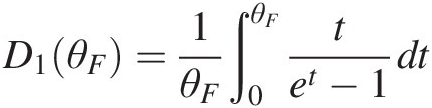 .
.
1. Construct the Q-Q plot of nonparametric and parametric Kendall distributions.
Applying Equation (4.20), the parametric Kendall distribution for the Gumbel–Hougaard, Clayton, and Frank copulas may be written as follows:
ϕt=−lntθ;ϕ’t=−θ−lntθ−1t;Kt=t−ϕtϕ′t=tθ−lntθ (4.21)
ϕt=1θt−θ−1;ϕ′t=−t−θ−1;Kt=t−ϕtϕ′t=t−tθ+1−tθ (4.22)
ϕt=−lne−θt−1e−θ−1;ϕ′t=θe−θte−θt−1;Kt=t+eθtlne−θt−1e−θ−1e−θt−1θ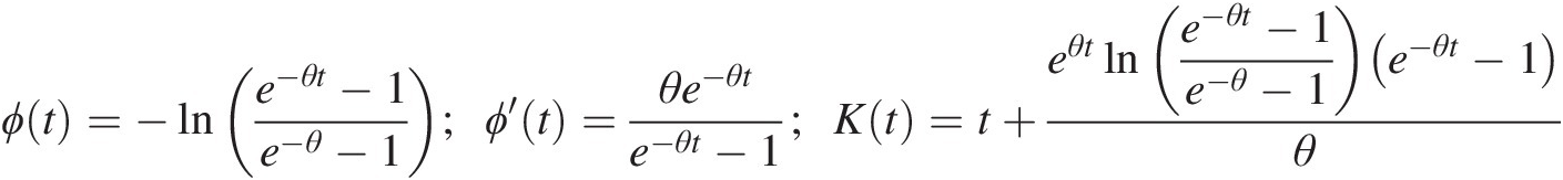 (4.23)
Table 4.8 lists the nonparametric and parametric Kendall distributions computed using the sample data. Figure 4.2 plots the nonparametric and parametric Kendall distributions. To illustrate how to obtain the results listed in Table 4.8, we will use {(x1, y1) :(11.68, 7.67)}x1y1:11.687.67 as an example.
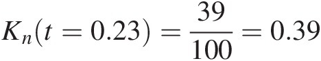
Compare {(x1, y1) : (11.68, 7.67)}x1y1:11.687.67 with all other bivariate pairs. We have (x3, y3 < (x1, y1), (x5, y5) < (x1, y1), …, (x96, y96) < (x1, y1)(x3,y3)<x1y1,x5y5<x1y1,…,x96y96<x1y1 with the total number of 23. Applying Equation (4.19) we have z1 = 23/(100 − 1)≈0.23z1=23/100−1≈0.23. Following the same procedure, we can compute z2, …, z100z2,…,z100. Applying Equation (4.19), Knt=0.23=39100=0.39
 .
.
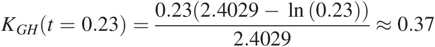
Now applying the Kendall distribution equations just derived for the Gumbel–Hougaard, Clayton, and Frank copulas using z1 = 23/(100 − 1)≈0.23z1=23/100−1≈0.23, we have the following:
Gumbel–Houggard: KGHt=0.23=0.232.4029−ln0.232.4029≈0.37
Clayton: KCt=0.23=t−tθ+1−tθ=0.23−0.232.8058+1−0.232.8058≈0.31

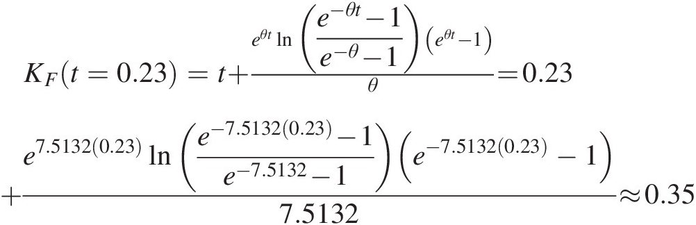
Frank: KFt=0.23=t+eθtlne−θt−1e−θ−1eθt−1θ=0.23+e7.51320.23lne−7.51320.23−1e−7.5132−1e−7.51320.23−17.5132≈0.35
2. Construct the K-plot for bivariate sample data. Following Example 3.17 and using Equations (3.81) introduced in Section 3.4.4, the K-plot of the bivariate sample data is shown in Figure 4.3.
3. Construct the chi-plot for the bivariate sample data. Following Example 3.16 and using Equations (3.77)–(3.80) introduced in Section 3.4.3, the chi-plot is shown in Figure 4.3.
Now from this example, we can reach the following conclusions:
The empirical Kendall correlation coefficient calculated, K-plot, and chi-plot in Figure 4.3 graphically indicate the positive dependence of the bivariate sample data.
From the Q-Q plots (Figure 4.2), graphically the Gumbel–Hougaard and Frank copulas seem to have a better fit than does the Clayton copula in the case of modeling the bivariate sample data.


Table 4.8. Nonparametric and parametric estimates of the Kendall distribution.
| No. | X | Y | Vi | Kn | Gumbel– Hougaard | Clayton | Frank |
|---|---|---|---|---|---|---|---|
| 1 | 11.68 | 7.67 | 0.24 | 0.39 | 0.38 | 0.32 | 0.36 |
| 2 | 18.01 | 15.54 | 0.88 | 0.95 | 0.93 | 0.97 | 0.96 |
| 3 | 9.15 | 3.03 | 0.05 | 0.08 | 0.11 | 0.07 | 0.12 |
| 4 | 16.56 | 12.49 | 0.73 | 0.81 | 0.83 | 0.88 | 0.85 |
| 5 | 7.80 | 7.41 | 0.14 | 0.24 | 0.25 | 0.19 | 0.25 |
| 6 | 13.11 | 6.36 | 0.17 | 0.28 | 0.30 | 0.23 | 0.28 |
| 7 | 9.81 | 8.03 | 0.26 | 0.41 | 0.41 | 0.35 | 0.38 |
| 8 | 11.76 | 11.63 | 0.48 | 0.64 | 0.63 | 0.63 | 0.61 |
| 9 | 20.59 | 16.60 | 0.96 | 0.99 | 0.98 | 1.00 | 0.99 |
| 10 | 21.60 | 16.00 | 0.95 | 0.98 | 0.97 | 1.00 | 0.99 |
| 11 | 7.05 | 8.00 | 0.07 | 0.15 | 0.15 | 0.09 | 0.15 |
| 12 | 16.44 | 14.32 | 0.82 | 0.88 | 0.89 | 0.94 | 0.92 |
| 13 | 16.91 | 16.68 | 0.88 | 0.95 | 0.93 | 0.97 | 0.96 |
| 14 | 13.94 | 13.28 | 0.70 | 0.79 | 0.80 | 0.86 | 0.82 |
| 15 | 12.74 | 10.81 | 0.51 | 0.69 | 0.65 | 0.66 | 0.64 |
| 16 | 10.75 | 10.43 | 0.36 | 0.52 | 0.51 | 0.48 | 0.49 |
| 17 | 8.63 | 8.37 | 0.21 | 0.35 | 0.35 | 0.28 | 0.33 |
| 18 | 26.09 | 20.42 | 1.00 | 1.00 | 1.00 | 1.00 | 1.00 |
| 19 | 8.47 | 6.47 | 0.11 | 0.21 | 0.21 | 0.15 | 0.21 |
| 20 | 18.33 | 14.25 | 0.85 | 0.92 | 0.91 | 0.96 | 0.94 |
| 21 | 7.28 | 5.30 | 0.06 | 0.12 | 0.13 | 0.08 | 0.14 |
| 22 | 18.81 | 13.14 | 0.78 | 0.85 | 0.86 | 0.92 | 0.89 |
| 23 | 8.63 | 9.70 | 0.25 | 0.40 | 0.39 | 0.34 | 0.37 |
| 24 | 18.29 | 16.51 | 0.91 | 0.96 | 0.95 | 0.99 | 0.98 |
| 25 | 17.24 | 10.94 | 0.61 | 0.74 | 0.74 | 0.77 | 0.74 |
| 26 | 20.95 | 13.47 | 0.80 | 0.87 | 0.87 | 0.93 | 0.90 |
| 27 | 8.65 | 7.91 | 0.19 | 0.32 | 0.32 | 0.26 | 0.31 |
| 28 | 6.84 | 7.13 | 0.06 | 0.12 | 0.13 | 0.08 | 0.14 |
| 29 | 8.40 | 9.02 | 0.20 | 0.34 | 0.33 | 0.27 | 0.32 |
| 30 | 11.32 | 10.79 | 0.41 | 0.59 | 0.56 | 0.54 | 0.54 |
| 31 | 11.69 | 9.16 | 0.36 | 0.52 | 0.51 | 0.48 | 0.49 |
| 32 | 12.80 | 11.71 | 0.59 | 0.73 | 0.72 | 0.75 | 0.72 |
| 33 | 7.07 | 1.34 | 0.01 | 0.03 | 0.03 | 0.01 | 0.04 |
| 34 | 7.96 | 11.08 | 0.19 | 0.32 | 0.32 | 0.26 | 0.31 |
| 35 | 4.76 | 2.34 | 0.01 | 0.03 | 0.03 | 0.01 | 0.04 |
| 36 | 9.18 | 7.98 | 0.23 | 0.37 | 0.37 | 0.31 | 0.35 |
| 37 | 14.80 | 12.87 | 0.71 | 0.80 | 0.81 | 0.87 | 0.83 |
| 38 | 8.95 | 7.27 | 0.16 | 0.26 | 0.28 | 0.22 | 0.27 |
| 39 | 18.26 | 15.09 | 0.87 | 0.93 | 0.92 | 0.97 | 0.95 |
| 40 | 5.92 | 3.40 | 0.04 | 0.06 | 0.09 | 0.05 | 0.10 |
| 41 | 11.51 | 14.23 | 0.50 | 0.68 | 0.64 | 0.65 | 0.63 |
| 42 | 9.32 | 11.75 | 0.33 | 0.46 | 0.48 | 0.44 | 0.46 |
| 43 | 13.23 | 8.15 | 0.34 | 0.48 | 0.49 | 0.46 | 0.47 |
| 44 | 10.71 | 12.36 | 0.42 | 0.60 | 0.57 | 0.56 | 0.55 |
| 45 | 11.50 | 5.75 | 0.12 | 0.22 | 0.23 | 0.16 | 0.22 |
| 46 | 7.63 | 4.57 | 0.07 | 0.15 | 0.15 | 0.09 | 0.15 |
| 47 | 7.67 | 6.78 | 0.11 | 0.21 | 0.21 | 0.15 | 0.21 |
| 48 | 8.55 | 10.54 | 0.23 | 0.37 | 0.37 | 0.31 | 0.35 |
| 49 | 8.32 | 7.97 | 0.17 | 0.28 | 0.30 | 0.23 | 0.28 |
| 50 | 10.36 | 13.48 | 0.40 | 0.58 | 0.55 | 0.53 | 0.53 |
| 51 | 12.82 | 6.28 | 0.15 | 0.25 | 0.27 | 0.20 | 0.26 |
| 52 | 7.79 | 7.49 | 0.14 | 0.24 | 0.25 | 0.19 | 0.25 |
| 53 | 16.02 | 13.94 | 0.79 | 0.86 | 0.87 | 0.93 | 0.90 |
| 54 | 14.03 | 12.99 | 0.70 | 0.79 | 0.80 | 0.86 | 0.82 |
| 55 | 8.53 | 8.46 | 0.20 | 0.34 | 0.33 | 0.27 | 0.32 |
| 56 | 10.45 | 9.44 | 0.32 | 0.45 | 0.47 | 0.43 | 0.45 |
| 57 | 18.71 | 13.97 | 0.83 | 0.89 | 0.89 | 0.95 | 0.93 |
| 58 | 13.60 | 10.89 | 0.57 | 0.71 | 0.70 | 0.73 | 0.70 |
| 59 | 9.02 | 15.45 | 0.31 | 0.43 | 0.46 | 0.42 | 0.44 |
| 60 | 12.05 | 2.15 | 0.03 | 0.05 | 0.07 | 0.04 | 0.08 |
| 61 | 12.65 | 11.01 | 0.49 | 0.66 | 0.64 | 0.64 | 0.62 |
| 62 | 10.79 | 7.24 | 0.18 | 0.30 | 0.31 | 0.24 | 0.29 |
| 63 | 11.24 | 9.48 | 0.35 | 0.49 | 0.50 | 0.47 | 0.48 |
| 64 | 12.66 | 10.39 | 0.45 | 0.61 | 0.60 | 0.59 | 0.58 |
| 65 | 10.56 | 9.77 | 0.34 | 0.48 | 0.49 | 0.46 | 0.47 |
| 66 | 15.56 | 13.47 | 0.74 | 0.83 | 0.83 | 0.89 | 0.85 |
| 67 | 15.74 | 13.64 | 0.78 | 0.85 | 0.86 | 0.92 | 0.89 |
| 68 | 16.45 | 16.24 | 0.84 | 0.91 | 0.90 | 0.96 | 0.93 |
| 69 | 7.64 | 6.57 | 0.10 | 0.19 | 0.20 | 0.14 | 0.20 |
| 70 | 6.37 | 6.31 | 0.05 | 0.08 | 0.11 | 0.07 | 0.12 |
| 71 | 10.36 | 11.21 | 0.37 | 0.54 | 0.52 | 0.49 | 0.50 |
| 72 | 8.59 | 6.05 | 0.10 | 0.19 | 0.20 | 0.14 | 0.20 |
| 73 | 16.45 | 12.99 | 0.74 | 0.83 | 0.83 | 0.89 | 0.85 |
| 74 | 5.72 | 1.37 | 0.01 | 0.03 | 0.03 | 0.01 | 0.04 |
| 75 | 14.38 | 11.53 | 0.64 | 0.76 | 0.76 | 0.80 | 0.76 |
| 76 | 9.71 | 3.11 | 0.06 | 0.12 | 0.13 | 0.08 | 0.14 |
| 77 | 12.75 | 9.22 | 0.39 | 0.57 | 0.54 | 0.52 | 0.52 |
| 78 | 10.29 | 8.66 | 0.30 | 0.42 | 0.45 | 0.40 | 0.43 |
| 79 | 13.01 | 10.17 | 0.47 | 0.63 | 0.62 | 0.62 | 0.60 |
| 80 | 8.09 | 8.65 | 0.18 | 0.30 | 0.31 | 0.24 | 0.29 |
| 81 | 7.06 | 7.38 | 0.07 | 0.15 | 0.15 | 0.09 | 0.15 |
| 82 | 13.63 | 10.13 | 0.49 | 0.66 | 0.64 | 0.64 | 0.62 |
| 83 | 12.76 | 11.56 | 0.57 | 0.71 | 0.70 | 0.73 | 0.70 |
| 84 | 7.86 | 5.65 | 0.09 | 0.16 | 0.18 | 0.12 | 0.18 |
| 85 | 20.31 | 15.68 | 0.93 | 0.97 | 0.96 | 0.99 | 0.98 |
| 86 | 7.14 | 10.80 | 0.10 | 0.19 | 0.20 | 0.14 | 0.20 |
| 87 | 12.06 | 11.11 | 0.50 | 0.68 | 0.64 | 0.65 | 0.63 |
| 88 | 15.57 | 11.14 | 0.63 | 0.75 | 0.75 | 0.79 | 0.75 |
| 89 | 13.75 | 10.87 | 0.58 | 0.72 | 0.71 | 0.74 | 0.71 |
| 90 | 7.36 | 3.41 | 0.06 | 0.12 | 0.13 | 0.08 | 0.14 |
| 91 | 13.09 | 14.23 | 0.66 | 0.77 | 0.77 | 0.82 | 0.78 |
| 92 | 10.13 | 11.91 | 0.37 | 0.54 | 0.52 | 0.49 | 0.50 |
| 93 | 12.71 | 10.50 | 0.47 | 0.63 | 0.62 | 0.62 | 0.60 |
| 94 | 9.84 | 10.00 | 0.32 | 0.45 | 0.47 | 0.43 | 0.45 |
| 95 | 16.82 | 14.32 | 0.84 | 0.91 | 0.90 | 0.96 | 0.93 |
| 96 | 5.78 | 2.57 | 0.03 | 0.05 | 0.07 | 0.04 | 0.08 |
| 97 | 15.61 | 8.97 | 0.39 | 0.57 | 0.54 | 0.52 | 0.52 |
| 98 | 10.96 | 7.91 | 0.24 | 0.39 | 0.38 | 0.32 | 0.36 |
| 99 | 11.83 | 9.14 | 0.36 | 0.52 | 0.51 | 0.48 | 0.49 |
| 100 | 11.93 | 9.42 | 0.38 | 0.55 | 0.53 | 0.51 | 0.51 |

Figure 4.2 Nonparametric and parametric Kendall distribution plots for bivariate random variables X and Y.

Figure 4.3 K-plot and chi-plot for the bivariate sample data.
4.5.2 MLE for Two- or d-Dimensional Symmetric Archimedean Copulas
In Section 3.6, we introduced three procedures to estimate the copula parameter θ using maximum likelihood estimation (MLE): (i) find the exact MLE in which the parameters of marginal distribution and copula function are estimated simultaneously using MLE; (ii) estimate the parameters for marginal distributions first and then estimate the copula parameter using the fitted marginal distributions using MLE, i.e., two-stage ML; and (iii) estimate the copula parameter directly from empirical marginal distributions using MLE. For the first and second marginal-dependent procedures, the copula function is more likely to be misidentified if the marginal distributions are misidentified. For the third marginal free procedure, the copula function is less likely to be misidentified. Table 4.3 lists the copula density functions needed for the parameter estimation using the maximum likelihood method. We present the parameter estimation using MLE with two examples.
Example 4.13 Using the same dataset as those in Example 4.12, estimate the copula parameters for the Gumbel–Hougaard, Clayton, Frank, and Joe copulas.
Solution: We will use all three procedures to estimate the copula parameters with the detailed derivation given for the Gumbel–Hougaard copula as an example.
Exact ML: From Table 4.3, we have the copula density function of the Gumbel–Hougaard copula as follows:
 (4.24)
Its logarithm can be written as follows:
 (4.25)
As shown in Table 4.8, X and Y follow the gamma and normal distributions, respectively, as follows:

Using Equations (3.97) and (3.98), we can rewrite the joint density function and its log-likelihood function as follows:
Let Θ = [α, β, μ, σ2, θ].Θ=αβμσ2θ. We have the following:
 (4.26)
Taking the partial derivative of logL(Θ)logLΘ with respect to parameter Θ = [α, β, μ, σ2, θ]Θ=αβμσ2θ and setting the derivative as zero, we can optimize the parameter as Θ̂=[α̂,β̂,μ̂,σ̂2,θ̂] .
.
Two-stage ML: To apply this method, first we estimate the parameters of marginal distributions using MLE. Second, let u1=F̂X(xα̂,β̂),u2=F̂Yyμ̂σ̂2, and substitute u1, u2u1,u2 into Equation (4.24). Third, optimize the log-likelihood function to estimate the copula parameter in which the log-likelihood function can be written as follows:
 (4.27)
Semiparametric ML: To apply the semiparametric ML method, first we need to calculate the empirical probability distribution. For example, the commonly applied Weibull plotting-position formula can be given as follows:
 (4.28)
Second, let u1 = Fn(x1), u2 = Fn(x2)u1=Fnx1,u2=Fnx2 and substitute u1, u2u1,u2 into Equation (4.24). Third, optimize the likelihood function as in the two-stage ML solution to estimate the copula parameter.
Table 4.9 lists the parameters estimated using all three procedures for the bivariate random variables.
Table 4.9. Parameters estimated using MLE.
| Methods | Copulas | Marginal distributions | Copula parameter: θθ | Log-likelihood | |
|---|---|---|---|---|---|
| X : (α, β)X:αβ | Y : (μ, σ2)Y:μσ2 | ||||
| Exact ML | Gumbel–Houggard | (8.408, 1.424) | (9.939, 3.7572) | 2.401 | –501.85 |
| Two-stage ML | (8.655, 1.379) | (9.944, 3.8532) | 2.037 | 52.837 | |
| Pseudo-ML | __ | __ | 2.390 | 48.578 | |
| Exact ML | Clayton | (8.381, 1.437) | (10.181, 4.1142) | 1.773 | –519.472 |
| Two-stage ML | (8.655, 1.379) | (9.944, 3.8532) | 2.439 | 47.931 | |
| Pseudo-ML | __ | __ | 1.712 | 33.844 | |
| Exact ML | Frank | (7.927, 1.534) | (10.195, 3.832) | 7.569 | –509.77 |
| Two-stage ML | (8.655, 1.379) | (9.944, 3.8532) | 10.155 | 72.455 | |
| Pseudo-ML | 7.474 | 43.775 | |||
| Exact ML | Joe | (7.945, 1.5) | (9.836, 3.8553) | 3.077 | –506.285 |
| Two-stage ML | (8.655, 1.379) | (9.944, 3.8532) | 2.068 | 41.44 | |
| Pseudo-ML | __ | __ | 2.952 | 43.776 | |
Example 4.14 Using the sample data given in Table 4.10: (1) estimate the trivariate copula parameters for the Clayton, Gumbel–Houggard, Frank, and Joe trivariate copula candidates using two-stage and semiparametric ML methods; (2) plot the empirical and parametric Kendall distributions.
Table 4.10. X, Y, Z sampled from gamma, exponential, and extreme value populations.
| No. | X | Y | Z | No. | X | Y | Z |
|---|---|---|---|---|---|---|---|
| 1 | 10.32 | 1.88 | 18.84 | 26 | 8.26 | 0.49 | 18.80 |
| 2 | 17.61 | 2.16 | 19.49 | 27 | 16.08 | 3.03 | 20.15 |
| 3 | 16.03 | 2.03 | 19.89 | 28 | 11.21 | 0.80 | 19.91 |
| 4 | 13.49 | 1.32 | 18.55 | 29 | 15.15 | 1.93 | 18.68 |
| 5 | 19.23 | 3.13 | 19.45 | 30 | 20.54 | 3.38 | 19.17 |
| 6 | 16.79 | 2.95 | 18.78 | 31 | 10.82 | 0.87 | 19.01 |
| 7 | 17.06 | 2.04 | 20.11 | 32 | 16.84 | 1.29 | 18.12 |
| 8 | 12.31 | 2.99 | 19.27 | 33 | 15.54 | 2.14 | 19.36 |
| 9 | 39.47 | 20.13 | 21.17 | 34 | 34.68 | 14.16 | 20.93 |
| 10 | 8.25 | 0.08 | 18.03 | 35 | 17.40 | 2.86 | 20.03 |
| 11 | 10.06 | 0.23 | 18.24 | 36 | 28.96 | 10.19 | 20.60 |
| 12 | 16.91 | 2.96 | 19.71 | 37 | 16.37 | 2.37 | 19.27 |
| 13 | 35.41 | 15.32 | 20.99 | 38 | 12.60 | 0.40 | 18.81 |
| 14 | 21.27 | 2.79 | 19.91 | 39 | 17.26 | 2.61 | 19.81 |
| 15 | 17.30 | 1.94 | 19.40 | 40 | 6.34 | 0.29 | 17.74 |
| 16 | 19.04 | 1.48 | 20.45 | 41 | 32.84 | 13.70 | 20.78 |
| 17 | 14.18 | 1.04 | 18.36 | 42 | 29.37 | 11.89 | 20.39 |
| 18 | 32.88 | 14.65 | 20.58 | 43 | 19.45 | 4.40 | 19.93 |
| 19 | 6.68 | 0.18 | 16.10 | 44 | 18.03 | 1.75 | 18.94 |
| 20 | 20.22 | 6.23 | 19.15 | 45 | 14.01 | 2.29 | 17.83 |
| 21 | 17.28 | 1.59 | 19.12 | 46 | 9.07 | 0.11 | 18.48 |
| 22 | 12.29 | 1.79 | 18.88 | 47 | 15.66 | 2.89 | 19.01 |
| 23 | 14.38 | 1.98 | 19.00 | 48 | 20.64 | 8.27 | 19.99 |
| 24 | 17.56 | 3.08 | 19.91 | 49 | 10.79 | 0.33 | 18.72 |
| 25 | 10.95 | 0.61 | 18.79 | 50 | 28.63 | 10.59 | 20.52 |
Solution: As discussed earlier, the Clayton copula can be extended to multivariate dimensions when θ>0θ>0 with strict generating function. The Gumbel–Hougaard and Joe bivariate copulas can be fully extended to multivariate dimensions with strict generating function in full parameter range. Even though the Frank copula also has strict generating function in full parameter range, the condition is only satisfied if θ>0θ>0. These multivariate copula functions are listed in Table 4.6.
1. Estimate the copula parameters using the two-stage and semiparametric ML methods.
The copula density function for each copula candidate can be written as follows:
Trivariate Clayton copula:
cθu1u2u3=2θ+1θ+1u1u2u3θ+1u1−θ+u2−θ+u3−θ1θ+3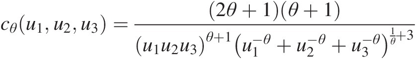 (4.29)
Trivariate Gumbel–Houggard copula:
cθu1u2u3=we−w11θw11θ(3θw11θ−3θ−3w11θ+w12θ+1)u1u2u3lnu1lnu2lnu3w13where: w = (−(lnu1)(lnu2)(lnu3))θ; w1 = (− ln u1)θ + (− ln u2)θ + (− ln u3)θw=−lnu1lnu2lnu3θ;w1=−lnu1θ+−lnu2θ+−lnu3θ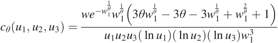 (4.30)
Trivariate Frank copula
cθu1u2u3=θ2e−θu1+u2+u3e−θ−12w1−3θ2we−θu1+u2+u3e−θ−14w12+2θ2w2we−θu1+u2+u3e−θ−16w13where: w=e−θu1−1e−θu2−1e−θu3−1;w1=we−θ−12+1 (4.31)
Trivariate Joe copula:
cθu1u2u3=θ2ww1+11θ−1+3θ2θ−1−1ww1w1+11θ−2+θ2θ−1−1θ−1−2ww12w1+11θ−3where: w = (1 − u1)θ − 1(1 − u2)θ − 1(1 − u3)θ − 1;w=1−u1θ−11−u2θ−11−u3θ−1;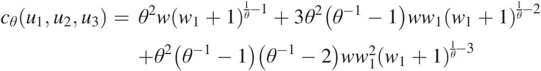 (4.32)
w1 = ((1 − u1)θ − 1)((1 − u2)θ − 1)((1 − u3)θ − 1)w1=1−u1θ−11−u2θ−11−u3θ−1
fxμσ=1σexpx−μσexp−expx−μσApplying the MLE for univariate probability distribution, the parameters are estimated and listed in Table 4.11.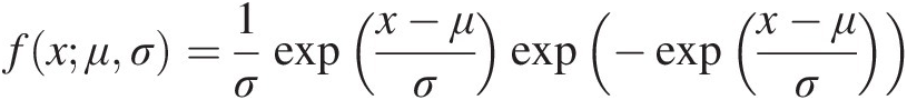 (4.33)


Table 4.11. Parameters estimated for random variables X, Y, and Z.
| X~Gamma (α, β)αβ | Y~Exponential (β)β | Z~Extreme value (μ, σ)μσ |
|---|---|---|
| (5.9251, 2.9824) | 3.9519 | (19.8077, 0.8634) |
Again, in the case of semiparametric ML method, the marginal probability is estimated nonparametrically using the Weibull plotting-position formula (i.e., Equation (4.28)). Table 4.12 lists the marginals computed parametrically and non-parametrically.
Table 4.12. Marginal distribution estimated parametrically and nonparametrically.
| No. | Random variables | Parametric | Nonparametric | ||||||
|---|---|---|---|---|---|---|---|---|---|
| X | Y | Z | F(x) | F(y) | F(z) | Fn(x) | Fn(y) | Fn(z) | |
| 1 | 10.32 | 1.88 | 18.84 | 0.15 | 0.38 | 0.28 | 0.14 | 0.37 | 0.31 |
| 2 | 17.61 | 2.16 | 19.49 | 0.55 | 0.42 | 0.50 | 0.67 | 0.51 | 0.59 |
| 3 | 16.03 | 2.03 | 19.89 | 0.46 | 0.40 | 0.67 | 0.43 | 0.45 | 0.65 |
| 4 | 13.49 | 1.32 | 18.55 | 0.31 | 0.28 | 0.21 | 0.29 | 0.27 | 0.18 |
| 5 | 19.23 | 3.13 | 19.45 | 0.63 | 0.55 | 0.48 | 0.73 | 0.75 | 0.57 |
| 6 | 16.79 | 2.95 | 18.78 | 0.51 | 0.53 | 0.26 | 0.49 | 0.65 | 0.24 |
| 7 | 17.06 | 2.04 | 20.11 | 0.52 | 0.40 | 0.76 | 0.55 | 0.47 | 0.78 |
| 8 | 12.31 | 2.99 | 19.27 | 0.25 | 0.53 | 0.41 | 0.25 | 0.69 | 0.49 |
| 9 | 39.47 | 20.13 | 21.17 | 0.99 | 0.99 | 0.99 | 0.98 | 0.98 | 0.98 |
| 10 | 8.25 | 0.08 | 18.03 | 0.07 | 0.02 | 0.12 | 0.06 | 0.02 | 0.08 |
| 11 | 10.06 | 0.23 | 18.24 | 0.13 | 0.06 | 0.15 | 0.12 | 0.08 | 0.12 |
| 12 | 16.91 | 2.96 | 19.71 | 0.51 | 0.53 | 0.59 | 0.53 | 0.67 | 0.61 |
| 13 | 35.41 | 15.32 | 20.99 | 0.98 | 0.98 | 0.98 | 0.96 | 0.96 | 0.96 |
| 14 | 21.27 | 2.79 | 19.91 | 0.73 | 0.51 | 0.68 | 0.82 | 0.59 | 0.71 |
| 15 | 17.30 | 1.94 | 19.40 | 0.53 | 0.39 | 0.46 | 0.61 | 0.41 | 0.55 |
| 16 | 19.04 | 1.48 | 20.45 | 0.63 | 0.31 | 0.88 | 0.71 | 0.29 | 0.84 |
| 17 | 14.18 | 1.04 | 18.36 | 0.35 | 0.23 | 0.17 | 0.33 | 0.24 | 0.14 |
| 18 | 32.88 | 14.65 | 20.58 | 0.97 | 0.98 | 0.91 | 0.92 | 0.94 | 0.88 |
| 19 | 6.68 | 0.18 | 16.10 | 0.03 | 0.04 | 0.01 | 0.04 | 0.06 | 0.02 |
| 20 | 20.22 | 6.23 | 19.15 | 0.68 | 0.79 | 0.37 | 0.76 | 0.80 | 0.45 |
| 21 | 17.28 | 1.59 | 19.12 | 0.53 | 0.33 | 0.36 | 0.59 | 0.31 | 0.43 |
| 22 | 12.29 | 1.79 | 18.88 | 0.24 | 0.36 | 0.29 | 0.24 | 0.35 | 0.33 |
| 23 | 14.38 | 1.98 | 19.00 | 0.37 | 0.39 | 0.32 | 0.35 | 0.43 | 0.37 |
| 24 | 17.56 | 3.08 | 19.91 | 0.55 | 0.54 | 0.67 | 0.65 | 0.73 | 0.69 |
| 25 | 10.95 | 0.61 | 18.79 | 0.17 | 0.14 | 0.26 | 0.20 | 0.18 | 0.25 |
| 26 | 8.26 | 0.49 | 18.80 | 0.07 | 0.12 | 0.27 | 0.08 | 0.16 | 0.27 |
| 27 | 16.08 | 3.03 | 20.15 | 0.47 | 0.54 | 0.77 | 0.45 | 0.71 | 0.80 |
| 28 | 11.21 | 0.80 | 19.91 | 0.19 | 0.18 | 0.67 | 0.22 | 0.20 | 0.67 |
| 29 | 15.15 | 1.93 | 18.68 | 0.41 | 0.39 | 0.24 | 0.37 | 0.39 | 0.20 |
| 30 | 20.54 | 3.38 | 19.17 | 0.70 | 0.57 | 0.38 | 0.78 | 0.76 | 0.47 |
| 31 | 10.82 | 0.87 | 19.01 | 0.17 | 0.20 | 0.33 | 0.18 | 0.22 | 0.39 |
| 32 | 16.84 | 1.29 | 18.12 | 0.51 | 0.28 | 0.13 | 0.51 | 0.25 | 0.10 |
| 33 | 15.54 | 2.14 | 19.36 | 0.43 | 0.42 | 0.45 | 0.39 | 0.49 | 0.53 |
| 34 | 34.68 | 14.16 | 20.93 | 0.98 | 0.97 | 0.97 | 0.94 | 0.92 | 0.94 |
| 35 | 17.40 | 2.86 | 20.03 | 0.54 | 0.52 | 0.73 | 0.63 | 0.61 | 0.76 |
| 36 | 28.96 | 10.19 | 20.60 | 0.93 | 0.92 | 0.92 | 0.86 | 0.84 | 0.90 |
| 37 | 16.37 | 2.37 | 19.27 | 0.48 | 0.45 | 0.41 | 0.47 | 0.55 | 0.51 |
| 38 | 12.60 | 0.40 | 18.81 | 0.26 | 0.10 | 0.27 | 0.27 | 0.14 | 0.29 |
| 39 | 17.26 | 2.61 | 19.81 | 0.53 | 0.48 | 0.63 | 0.57 | 0.57 | 0.63 |
| 40 | 6.34 | 0.29 | 17.74 | 0.02 | 0.07 | 0.09 | 0.02 | 0.10 | 0.04 |
| 41 | 32.84 | 13.70 | 20.78 | 0.97 | 0.97 | 0.95 | 0.90 | 0.90 | 0.92 |
| 42 | 29.37 | 11.89 | 20.39 | 0.93 | 0.95 | 0.86 | 0.88 | 0.88 | 0.82 |
| 43 | 19.45 | 4.40 | 19.93 | 0.65 | 0.67 | 0.68 | 0.75 | 0.78 | 0.73 |
| 44 | 18.03 | 1.75 | 18.94 | 0.57 | 0.36 | 0.31 | 0.69 | 0.33 | 0.35 |
| 45 | 14.01 | 2.29 | 17.83 | 0.34 | 0.44 | 0.10 | 0.31 | 0.53 | 0.06 |
| 46 | 9.07 | 0.11 | 18.48 | 0.09 | 0.03 | 0.19 | 0.10 | 0.04 | 0.16 |
| 47 | 15.66 | 2.89 | 19.01 | 0.44 | 0.52 | 0.33 | 0.41 | 0.63 | 0.41 |
| 48 | 20.64 | 8.27 | 19.99 | 0.70 | 0.88 | 0.71 | 0.80 | 0.82 | 0.75 |
| 49 | 10.79 | 0.33 | 18.72 | 0.17 | 0.08 | 0.25 | 0.16 | 0.12 | 0.22 |
| 50 | 28.63 | 10.59 | 20.52 | 0.92 | 0.93 | 0.90 | 0.84 | 0.86 | 0.86 |
Finally, maximizing the log-likelihood function of copula density functions, we are able to estimate the parameters for each copula candidate given in Table 4.13.
From Equation (4.11), the parametric Kendall distribution for trivariate Archimedean copula may be simplified as follows:
 (4.34)
Now, substituting the generating functions for Clayton, Gumbel–Houggard, Frank, and Joe copulas into Equation (4.34), we obtain the Kendall distribution function as follows:
Trivariate Clayton copula:
KCt=t+tt2θ−4tθ+32θ+ttθ−122θ2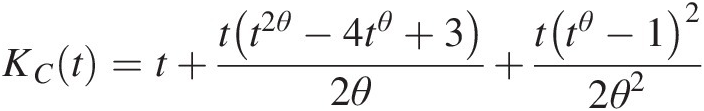 (4.35)
Trivariate Gumbel–Houggard copula:
KCt=t2θ2−3θlnt+ln2t+lnt2θ2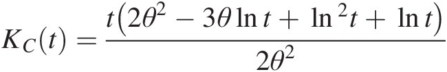 (4.36)
Trivariate Frank copula:
KCt=t+1−eθtθlne−θt−1e−θ−1−eθt−e2θt2θlne−θt−1e−θ−12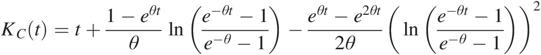 (4.37)
Trivariate Joe copula:
KCt=t+s1s21−t1−θθ+s22s131−t3−3θθ21−t2θ−2s12−θθ−11−tθ−2s12θ3where: s1 = (1 − t)θ − 1, s2 = ln (1 − (1 − t)θ)s1=1−tθ−1,s2=ln1−1−tθ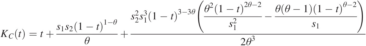 (4.38)


Table 4.13. Copula parameters estimated for trivariate analysis.
| Clayton θ, logL | Gumbel–Houggard θ, logL | Frank θ, logL | Joe θ, logL | |
|---|---|---|---|---|
| Two-stage | 2.112, 52.034 | 3.132, 86.533 | 9.796, 71.995 | 4.252, 80.813 |
| Semiparametric | 2.042, 49.606 | 3.034, 76.136 | 8.673, 60.927 | 4.213, 73.519 |
According to Equation (4.19) in Section 4.5.1, the nonparametric estimation of Kendall distribution can be given as follows:
i. Obtain zi=∑j=1n1x1j≤x1ix2j≤x2ix3j≤x3in−1;i=1,…,n,j≠i

ii. Construct Knz=∑i=1n1zi≤zn


Using the fitted copula parameter given in Table 4.13, Figures 4.4 and 4.5 plot the nonparametric and parametric Kendall distributions using the parameters estimated with two-stage and pseudo-MLE, respectively. From Figures 4.4 and 4.5, we see that nonparametric and parametric Kendall distributions have the best match for the Gumbel–Hougaard copula.

Figure 4.4 Comparison of nonparametric and parametric Kendall distributions with parameters estimated using two-stage MLE.

Figure 4.5 Comparison of nonparametric and parametric Kendall distributions with parameters estimated using pseudo-MLE.
4.6 Simulation of Symmetric Archimedean Copulas
In Section 3.7, we discussed the general procedure to simulate the random variables from any given copula function. For the symmetric Archimedean copulas, the simulation procedure can be revised based on the general simulation technique as follows.
Let the joint distribution multivariate random variables (x1, x2, …, xd)x1x2…xd be modeled by a symmetric Archimedean copula with generating function ϕϕ. Then we have the following:
Let u1 = FX1(x1), …, ud = FXd(xd)u1=FX1x1,…,ud=FXdxd, and the copula function can be written using the generating function ϕϕ as follows:
From the definition of the copula discussed in Section 3.1, we also have the following:
Let the conditional distribution of UiUi, given the values of U1, …, Ui − 1U1,…,Ui−1, be
 (4.41)
Substituting Equation (4.40) into Equation (4.41) and applying the associative property of the symmetric Archimedean copulas, we have the following:
 (4.42)
where ti=ϕu1+ϕu2+⋯+ϕui=∑k=1iϕuk;ϕ−1i−1ti=∂i−1ϕ−1ti∂tii−1,i=2,…,d Obviously, in Equations (4.41) and (4.42), the (partial) derivative exists for both the numerator and the denominator. More specifically, the (partial) derivative of the denominator is not zero.
Following the preceding derivation, the general simulation algorithm can be written as follows:
1. Simulate a d-independent random variable (v1, v2, …, vd)v1v2…vd from the uniform distribution U(0, 1)U01.
2. Set u1 = v1u1=v1.
3. Set v2=C2u2U1=u1=ϕ−11t2ϕ−11t1
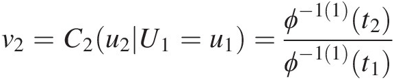 ; t1 = ϕ(u1), t2 = ϕ(u1) + ϕ(u2)t1=ϕu1,t2=ϕu1+ϕu2. Solve for u2u2 using the equation v2=ϕ−11t2ϕ−11t1
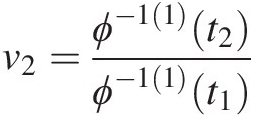 .
.
4. Set v3=C3u3U1=u1U2=u2=ϕ−12t3ϕ−12t2;t3=ϕu1+ϕu2+ϕu3
 and t2 = ϕ(u1) + ϕ(u2),t2=ϕu1+ϕu2. Solve for u3u3 using the equation v3=ϕ−12t3ϕ−12t2
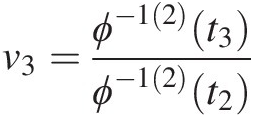 .
.
… …
5. Set vd=CdudU1=u1…Ud=ud=ϕ−1d−1tdϕ−1d−1td−1;td−1=ϕu1+ϕu2+…+ϕud−1,td=ϕu1+ϕu2+…+ϕud.
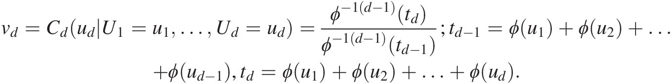 Solve for udud using vd=ϕ−1d−1tdϕ−1d−1td−1
 .
.


Here we summarize ϕ−1(2)(t)ϕ−12t of the Gumbel–Hougaard, Frank, Clayton, and Ali–Mikail–Haq copulas:
The generating function of the Gumbel–Houggard copula is given by ϕ(t) = (− ln (t))θϕt=−lntθ. Hence,
ϕ−1t=e−t1θ (4.43a)
ϕ−11=−t1θ−1e−t1θθ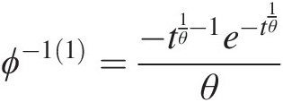 (4.43b)
ϕ−12=t2θ−2e−t1θ−1−θt1θ−2e−t−1θθ2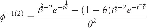 (4.43c)
Frank copula
The generating function of the Frank copula is given by ϕt=−lne−θu−1e−θ−1
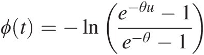 . Hence,
ϕ−1t=−1θln1+e−te−θ−1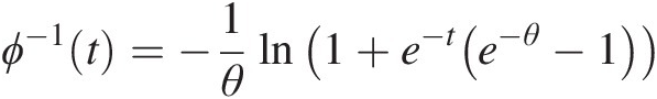 (4.44a)
ϕ−11t=e−te−θ−1θe−te−θ−1+1 (4.44b)
ϕ−12t=e−2te−θ−12θe−te−θ−1+12−e−te−θ−1θe−te−θ−1+1 (4.44c)
The generating function of the Clayton copula is given by ϕt=1θt−θ−1
 . Hence,
ϕ−1t=θt+1−1θ (4.45a)
ϕ−11t=−θt+1−1θ−1 (4.45b)
ϕ−12t=θ+1θt+1^−1θ−2 (4.45c)
The generating function of the Ali–Mikail–Haq copula is given by ϕt=ln1−θ1−tt
 . Hence, we have the following:
ϕ−1t=etθ−1θ−et2 (4.46a)
ϕ−11t=etθ−1θ−et2 (4.46b)
ϕ−12t=etθ−1θ+etθ−et3 (4.46c)


Example 4.15 Show how to generate the random variable for the bivariate (trivariate) Joe copula using the simulation procedure discussed previously.
Solution: The generating function of Joe copula is written as follows: ϕ(t) = − ln (1 − (1 − t)θ)ϕt=−ln1−1−tθ. Hence, the inverse of ϕϕ can be written as follows: ϕ−1t=1−1−expt1θ .
.
Bivariate case:
1. Generate two independent random variables [v1, v2]v1v2 from U(0, 1)U01.
2. Set u1 = v1u1=v1.
3. Set v2=ϕ−11t2ϕ−11t1
 , and we have the following:
ϕ−11t=∂−1ϕt∂t=exp−tθ1−exp−t1θ−1 (4.47)
4. Let t1 = − ln (1 − (1 − u1)θ), t2 = − ln (1 − (1 − u1)θ) − ln (1 − (1 − u2)θ).t1=−ln1−1−u1θ,t2=−ln1−1−u1θ−ln1−1−u2θ. Then we have the following:
ϕ−11t1=1−u1θ−11−u1θ1θ−1θ (4.48a)


 (4.48b)
 (4.48c)
Now u2 can be calculated numerically.
Trivariate case:
1. Generate independent random variables [v1, v2, v3]v1v2v3 from U(0, 1)U01.
2. Use Equation (4.48c) to numerically calculate u2.
3. For the trivariate case, we need to determine ϕ−1(2)(t)ϕ−12t, which is given as follows:
ϕ−12t=∂2ϕ−1t∂t2=1−exp−t1θθexpt−1θ2expt−12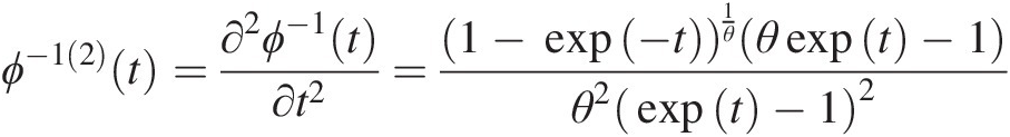 (4.49)
4. Let t3 = − ln (1 − (1 − u1)θ) − ln (1 − (1 − u2)θ) − ln (1 − (1 − u3)θ)t3=−ln1−1−u1θ−ln1−1−u2θ−ln1−1−u3θ, and we have the following:
ϕ−12t2=1−u¯1θ1−u¯2θ(θ−1−u¯1θ1−u¯2θu¯1θ−u¯1θu¯2θ+u¯2θ1/θθ2u¯1θ−u¯1θu¯2θ+u¯2θ2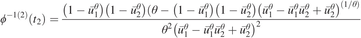 (4.49a)
ϕ−12t3=1−u¯1θ1−u¯2θ1−u¯3θθ−1−u¯1θ1−u¯2θ1−u¯3θ1−1−u¯1θ1−u¯2θ1−u¯3θ1θθ21−1−u¯1θ1−u¯2θ1−u¯3θ2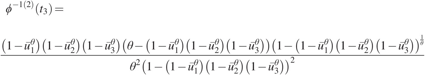 (4.49b)
v3=1−u¯3θθ−1−u¯1θ1−u¯2θ1−u¯3θθ1−u¯1θ1−u¯2θ1−1−u¯1θ1−u¯2θ1−u¯3θu¯1θ−u¯1θu¯2θ+u¯2θ1θ−2where, in Equations (4.49a)–(4.49c): u¯1=1−u1,u¯2=1−u2,u¯3=1−u3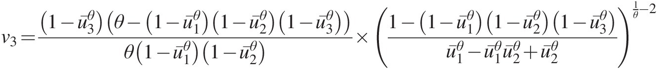 (4.49c)
 .
.


Now u3u3 can be calculated numerically.
Example 4.16 Simulate bivariate random variables (sample size of 200) with the parameters estimated in Example 4.13 based on the semiparametric ML method for the Gumbel–Hougaard and Frank copulas, and compare the simulated random variables with the empirical marginal variables.
Solution: According to the previous discussion of the Gumbel–Hougaard (Equations (4.43a) and (4.43b)) and Frank (Equations (4.44a) and (4.44b)) copulas, we can generate the bivariate random variables with the fitted parameter using the simulation procedure for symmetric Archimedean copulas. Here we will illustrate the simulation procedure using the Gumbel–Hougaard copula as an example:
1. Generate two independent, uniformly distributed variables
One can generate the independent, uniformly distributed random variables using the rand function in MATLAB:
[v1, v2] = rand (2, 1)v1v2=rand21, and we have: [v1, v2] = [0.1270, 0.9134]v1v2=0.12700.9134.
Notice that the random variables generated are subjected to change for each generation.
2. Set u1 = v1 = 0.1270, C(u2| u1) = v2 = 0.9134u1=v1=0.1270,Cu2u1=v2=0.9134.
Substituting Equations (4.43a)–(4.43b) into Equation (4.42), we have the following:
Cu2u1=ϕ−11t2ϕ−11t1=t11−1θet11/θt21θ−1e−t21θ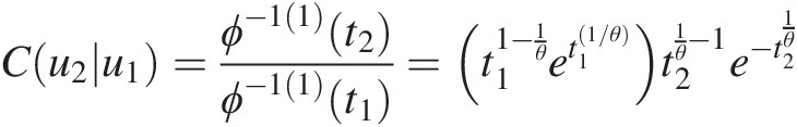

Applying θ = 2.39θ=2.39, we have the following:


Now we need to solve for t2. It is seen that the preceding equation does not have a closed-form inverse, and we will need to solve the equation numerically. In MATLAB, we can use the fsolve function to solve the general function of f(x) = 0fx=0. Thus, here we are solving f(t2) = C(u2| u1) − 0.9134 = 0ft2=Cu2u1−0.9134=0 as follows:
t2 = fsolve(@(t2)21.5534*t2^(1/2.39–1).*exp(-t2^(1/2.39))-0.9134,10), where @ is the function handle and 10 is the initial value. We obtain t2 = 6.0111t2=6.0111.
Applying t2 = ϕ(u1) + ϕ(u2)t2=ϕu1+ϕu2 we have the following: ϕ(u2) = t2 − ϕ(u1) = 6.0111 − 5.6486 = 0.3625ϕu2=t2−ϕu1=6.0111−5.6486=0.3625
Finally, we have u2=e−0.362512.39=0.5199 .
.
With the same procedure, we will be able to simulate the rest of the bivariate random variables.
Figure 4.6 compares simulated copula random variables with their corresponding empirical distributions. Figure 4.7 compares simulated X and Y from the fitted gamma and normal distributions (Table 4.9) with the sample random variables.

Figure 4.6 Comparison of simulated random variables with empirical marginal variables.

Figure 4.7 Comparison of simulated peak discharge and flood volume with observations.
From the simulation with Gumbel–Hougaard copula shown in Figures 4.6 and 4.7, we see that there exists an upper-tail dependence for the Gumbel–Hougaard copula and no visual effects of lower-tail dependence. From the simulation with Frank copula, we see that there does not exist significant dependence for either an upper- (upper-right corner) or a lower- (lower-left corner) tail dependence for the Frank copula.
Example 4.17 Simulate trivariate random variables (sample size of 200) with the parameters estimated in Example 4.14 based on the semiparametric ML for the Gumbel–Houggard and Clayton copulas, and compare the simulated random variables with the empirical marginal variables.
Solution: According to the general copula simulation procedure discussed in Equations (4.39)–(4.42), (4.43a)–(4.43c), (4.45a)–(4.45c) are derived from and can be applied to simulate the random variables from Gumbel–Houggard and Clayton copulas as follows: (1) generate independent trivariate random variables [v1, v2, v3]v1v2v3; (2) set u1 = v1u1=v1; (3) solve for u2u2 using u1, v2u1,v2, and Equation (4.43b) or Equation (4.45b); and (4) solve for u3u3 using u1, u2, v3u1,u2,v3, and Equation (4.43c) or Equation (4.45c). Here we will illustrate how to simulate the random variables with an example using the Clayton copula:
1. Generate three independent, uniformly distributed random variables:
Using the rand function to generate uniformly distributed random variables as follows: V=rand(3,1)
Then we have the following:
V=rand(3,1)
[v1, v2, v3] = [0.8147, 0.9058, 0.1270]v1v2v3=0.81470.90580.1270.
2. Set u1 = v1 = 0.8147u1=v1=0.8147 and solve u2u2 from v2 = C(u2| u1) = 0.9508v2=Cu2u1=0.9508. From the procedure described for the simulation for the Archimedean copulas, applying Equation (4.45a) with θ = 0.532θ=0.532, estimated using semiparametric MLE (or pseudo-MLE), we have the following:
t1=ϕu10.532=10.5320.8147−0.532−1=0.2165
t2 = ϕ(u1) + ϕ(u2) = 0.2165 + ϕ(u2)t2=ϕu1+ϕu2=0.2165+ϕu2
v2=ϕ−11t2ϕ−11t1=0.532t2+1−2.87970.5320.2165+1−2.8797=0.9058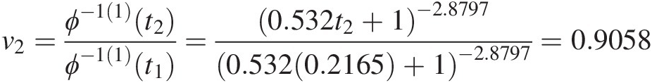
Finally, we can solve for u2u2 as follows: u2=0.5320.0733+1−10.532=0.9306
⇒ t2 = ϕ(u2) + 0.2165 = 0.2898 ⇒ ϕ(u2) = 0.2898 − 0.2165 = 0.0733⇒t2=ϕu2+0.2165=0.2898⇒ϕu2=0.2898−0.2165=0.0733
3. Now set u1 = 0.8147, u2 = 0.9306u1=0.8147,u2=0.9306 to solve for u3u3 from v3 = C(u3| U1 = u1, U2 = u2) = 0.1270v3=Cu3U1=u1U2=u2=0.1270. Applying Equation (4.45b), we have the following:
t2 = ϕ(u1) + ϕ(u2) = 0.2898t2=ϕu1+ϕu2=0.2898, which is computed from the previous step, and
t3 = ϕ(u3) + 0.2898t3=ϕu3+0.2898
v3=ϕ−12t3ϕ−12t2=0.532t3+1−10.532−20.5320.298+1−10.532−2=0.1270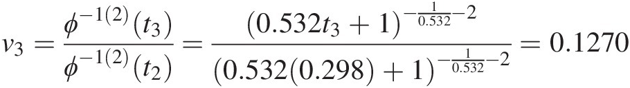
⇒t3 = 1.8131, u3 = 0.2810⇒t3=1.8131,u3=0.2810.


Similarly, one can perform the simulation using the Gumbel–Hougaard copula. Figure 4.8 plots the marginal random variables simulated from the copula function and empirical marginal random variables. Figure 4.9 plots the simulated random variables from the fitted marginal distributions and the samples given in Table 4.10.

Figure 4.8 Comparison of simulated trivariate random variables and empirical maginals.

Figure 4.9 Comparison of simulated trivariate random variables and samples.
We can see from Figure 4.8 that visually, the Clayton and Gumbel–Hougaard copulas have similar performance.
4.7 Goodness-of-Fit Statistics Test for Archimedean Copulas
Usually, the best-fitted copula is considered as the copula function with the largest log-likelihood. However, it is needed to further ensure the appropriateness of the chosen copula function with the use of the formal goodness-of-fit (GoF) test statistics besides the visual comparison. In Section 3.8, we introduced two of the most powerful GoF test statistics: SnB based on Rosenblatt’s transform and SnSn based on the empirical copula for bivariate random variables. Here, we will discuss the procedure to construct the goodness-of-fit test statistics SnB
 and SnSn for multivariate symmetric Archimedean copulas (i.e., d ≥ 3d≥3).
4.7.1 Goodness-of-Fit Statistics SnB for Multivariate Symmetric Archimedean Copulas

Let multivariate random variable X1, X2, …, XdX1,X2,…,Xd be modeled by the symmetric Archimedean copulas function Cθ(u1, …, ud); u1 = F1(x1), …, ud = Fd(xd)Cθu1…ud;u1=F1x1,…,ud=Fdxd; then, based on Rosenblatt’s transform, i.e., Equations (4.41) and (4.42), we have the following:
 (4.50)
Then Equation (3.122) is rewritten as follows:
 (4.51)
In the same way as the goodness-of-fit statistics test for bivariate case, Z1, …, ZdZ1,…,Zd should be “close” to independently uniformly distributed as C⊥C⊥. Then, according to Genest et al. (2007), Equation (3.123) for the construction of goodness-of-fit statistics can be rewritten as follows:
 (4.52)
The P-value of the statistics is again determined, based on the parametric bootstrap simulation, by simply extending the bivariate case to a multivariate case with the same simulation procedure, except that this case is in d dimension.
4.7.2 Goodness-of-Fit Statistic SnSn for Multivariate Symmetric Archimedean Copulas
Following Genest et al. (2007) and Genest and Rémillard (2008), again let multivariate random variables X1, …, XdX1,…,Xd be modeled by the symmetric Archimedean copula function: Cθ(u1, u2, …, ud); u1 = F1(x1), …, ud = Fd(xd)Cθu1u2…ud;u1=F1x1,…,ud=Fdxd.
The empirical d-dimensional copula function can be given as follows:
 (4.53)
Now the goodness-of-fit test statistic and the P-value can be estimated using the same procedure as that discussed in Section 3.8.1.
4.7.3 Goodness-of-Fit Test Statistic SnK Based on the Kendall Probability Transform

Besides the GoF statistics SnB,Sn ; SnK
; SnK are the test statistics based on the Kendall probability transform. It is a powerful and convenient test for the symmetric Archimedean copulas. In what follows, we discuss the procedure to construct SnK
 and the corresponding P-value based on the discussion in Genest et al. (2007).
Similar to the test statistics SnB and SnSn, its null hypothesis is that the fitted copula function (i.e., here fitted symmetric Archimedean copula function) can appropriately represent the multivariate distribution function of the multivariate random variable. In Section 4.1, we have introduced the Kendall distribution function KC(t)KCt(i.e., Equation (4.11)). Based on the Kendall distribution for bivariate and trivariate random variables introduced in Sections 4.5.1 and 4.5.2, the nonparametric Kendall distribution for multivariate random variable of d-dimension can be given as
 (4.54a)
 (4.54b)
Now the test statistic can be written as follows:
 (4.55)
where
 (4.55a)
Genest et al. (2007) showed that Equation (4.55) can be calculated as follows:
 (4.56)
Finally, with the fitted symmetric Achimedean copula, the P-value of the test statistic is again approximated using parametric bootstrap simulation as follows:
1. Generate a multivariate sample X1∗,…,Xd∗
 (with the same sample of the tested dataset) from the fitted Archimedean copula Cθ̂
 and compute their associated rank R1∗,…,Rd∗
 .
.
2. Estimate the copula parameter θ̂∗
 using R1∗n+1…Rd∗n+1
 .
.
3. Compute Kn∗
 using Equation (4.54) from the generated multivariate sample X1∗,…,Xd∗
 and SnK∗
 using Equation (4.56), replacing θ̂
 with θ̂∗
 .
.


Repeating steps 1 through 3 for a larger integer number N, we can approximate the P-value as follows:
 (4.57)
Example 4.18 Goodness-of-fit statistics.
In this example, we generate GoF statistics for both bivariate and trivariate cases:
Bivariate case: Compute the goodness-of-fit statistics SnB
 and SnSn, and the corresponding P-value using parametric bootstrap simulation for the parameters (the Gumbel–Hougaard and Frank copulas) estimated with semiparametric ML in Example 4.13.
Trivariate case: Compute the goodness-of-fit statistics SnK
 and the corresponding P-value using parametric bootstrap simulation for the parameters of the Gumbel–Houggard and Clayton copulas with semiparametric ML in Example 4.14.


Solution:
Bivariate case:
For bivariate random variables given in Example 4.13, we have estimated the parameters using the semiparametric ML as the Gumbel–Hougaard copula (θ = 2.390θ=2.390) and the Frank copula (θ = 7.474θ=7.474). Let u1 = FX(x), u2 = FY(y)u1=FXx,u2=FYy; we can construct test statistics for bivariate frequency analysis.
i. Goodness-of-fit statistics SnB
 for the Gumbel–Hougaard and Frank copulas:
From Equation (4.41), we have the following:
Gumbel–Hougaard copula:
Z1=u1Z2=ϕ−11∑i=12ϕu1+ϕu2ϕ−11ϕu1=e−−lnu1)θ+−lnu2θ1θ−lnu1θ−1−lnu1θ+−lnu2θ1θ−1u1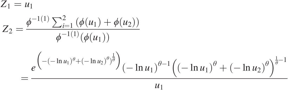 (4.58)
Frank copula:
Z1=u1Z2=ϕ−11∑i=12ϕu1+ϕu2ϕ−11ϕu1=e−θu1e−θu2−1e−θu1−1e−θu2−1e−θ−1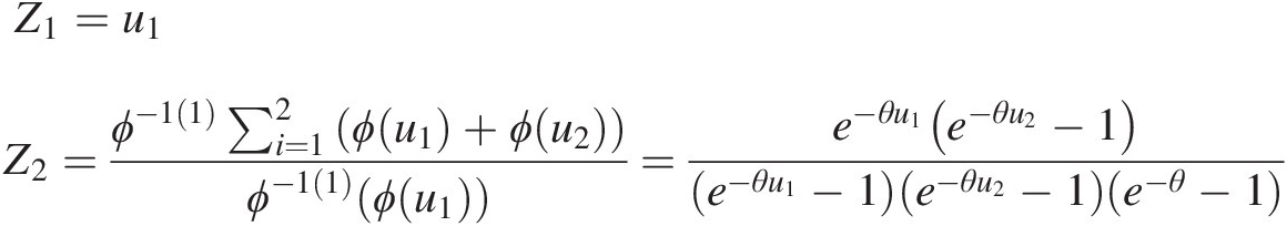 (4.59)
Now, we can compute {Z1, Z2}Z1Z2 using Equations (4.58) and (4.59) as shown in Table 4.14.
Inserting the computed {Z1, Z2}Z1Z2 into Equation (4.52), we can compute the test statistic SnB
 as follows:
Gumbel–Hougaard: SnB=0.0483
With 5,000 bootstrap parametric simulations as an example, the P-values can be approximated using the procedure discussed in Section 3.8.1, as follows:
PGumbel − Hougaard (θ = 2.390) = 0.202; PFrank(θ = 7.474) = 0.28PGumbel−Hougaardθ=2.390=0.202;PFrankθ=7.474=0.28
ii. Goodness-of-fit statistics SnSn for Gumbel–Hougaard and Frank copulas:
The empirical copula function is estimated using Equation (4.53) and the copula function, with the estimated parameter calculated using the Gumbel–Hougaard (Frank) copula function.
Now, the test statistics SnSn can be estimated as follows:
Gumbel–Hougaard: Sn = 0.0141Sn=0.0141
and Frank: Sn = 0.0153Sn=0.0153
With 5,000 bootstrap parametric simulations, the P-values can be approximated using the procedure discussed in Section 3.8.2, as follows:
PGumbel − Hougaard(θ = 1.889) = 0.714; PFrank(θ = 5.606) = 0.567PGumbel−Hougaardθ=1.889=0.714;PFrankθ=5.606=0.567
 (Rosenblatt transform) and SnSn (empirical copula). This is because the Frank copula cannot capture the upper-tail dependence embedded in the flood peak and flood volume (i.e., Figures 4.6 and 4.7).
Trivariate case:


From Example 4.14, we have estimated the copula parameters for trivariate flood frequency analysis using semiparametric ML as the Gumbel–Hougaard copula (θ = 1.368θ=1.368) and the Clayton copula (θ = 0.721θ=0.721). The corresponding Kendall distribution is given as Equation (4.32) for the Gumbel–Hougaard copula and Equation (4.31) for the Clayton copula. The test statistics are determined using Equations (4.51a)–(4.53). Table 4.15 lists the computed nonparametric and parametric Kendall distribution.
Table 4.14. {Z1, Z2}Z1Z2 computed from Equations (4.58) and (4.59).
| No. | Marginals | Gumbel–Hougaard | Frank | No | Marginals | Gumbel–Hougaard | Frank | ||||||
|---|---|---|---|---|---|---|---|---|---|---|---|---|---|
| Fn(x) | Fn(y) | Z1 | Z2 | Z1 | Z2 | Fn(x) | Fn(y) | Z1 | Z2 | Z1 | Z2 | ||
| 1 | 0.515 | 0.267 | 0.515 | 0.163 | 0.515 | 0.092 | 51 | 0.653 | 0.149 | 0.653 | 0.027 | 0.653 | 0.031 |
| 2 | 0.891 | 0.921 | 0.891 | 0.790 | 0.891 | 0.972 | 52 | 0.158 | 0.257 | 0.158 | 0.573 | 0.158 | 0.085 |
| 3 | 0.317 | 0.059 | 0.317 | 0.044 | 0.317 | 0.009 | 53 | 0.812 | 0.832 | 0.812 | 0.685 | 0.812 | 0.917 |
| 4 | 0.851 | 0.733 | 0.851 | 0.300 | 0.851 | 0.814 | 54 | 0.743 | 0.762 | 0.743 | 0.653 | 0.743 | 0.850 |
| 5 | 0.168 | 0.248 | 0.168 | 0.537 | 0.168 | 0.079 | 55 | 0.238 | 0.356 | 0.238 | 0.631 | 0.238 | 0.176 |
| 6 | 0.683 | 0.168 | 0.683 | 0.028 | 0.683 | 0.038 | 56 | 0.416 | 0.446 | 0.416 | 0.549 | 0.416 | 0.303 |
| 7 | 0.356 | 0.327 | 0.356 | 0.419 | 0.356 | 0.144 | 57 | 0.931 | 0.842 | 0.931 | 0.248 | 0.931 | 0.925 |
| 8 | 0.535 | 0.683 | 0.535 | 0.796 | 0.535 | 0.742 | 58 | 0.703 | 0.594 | 0.703 | 0.375 | 0.703 | 0.583 |
| 9 | 0.960 | 0.970 | 0.960 | 0.785 | 0.960 | 0.991 | 59 | 0.307 | 0.911 | 0.307 | 0.998 | 0.307 | 0.967 |
| 10 | 0.980 | 0.941 | 0.980 | 0.194 | 0.980 | 0.980 | 60 | 0.564 | 0.030 | 0.564 | 0.004 | 0.564 | 0.004 |
| 11 | 0.069 | 0.317 | 0.069 | 0.805 | 0.069 | 0.134 | 61 | 0.584 | 0.614 | 0.584 | 0.614 | 0.584 | 0.620 |
| 12 | 0.822 | 0.891 | 0.822 | 0.848 | 0.822 | 0.957 | 62 | 0.455 | 0.218 | 0.455 | 0.151 | 0.455 | 0.061 |
| 13 | 0.871 | 0.980 | 0.871 | 0.994 | 0.871 | 0.994 | 63 | 0.475 | 0.455 | 0.475 | 0.486 | 0.475 | 0.319 |
| 14 | 0.733 | 0.782 | 0.733 | 0.721 | 0.733 | 0.872 | 64 | 0.594 | 0.515 | 0.594 | 0.417 | 0.594 | 0.428 |
| 15 | 0.614 | 0.574 | 0.614 | 0.492 | 0.614 | 0.544 | 65 | 0.426 | 0.475 | 0.426 | 0.587 | 0.426 | 0.354 |
| 16 | 0.446 | 0.525 | 0.446 | 0.645 | 0.446 | 0.447 | 66 | 0.772 | 0.802 | 0.772 | 0.693 | 0.772 | 0.891 |
| 17 | 0.267 | 0.347 | 0.267 | 0.575 | 0.267 | 0.165 | 67 | 0.802 | 0.822 | 0.802 | 0.680 | 0.802 | 0.909 |
| 18 | 0.990 | 0.990 | 0.990 | 0.666 | 0.990 | 0.997 | 68 | 0.832 | 0.950 | 0.832 | 0.971 | 0.832 | 0.984 |
| 19 | 0.228 | 0.178 | 0.228 | 0.304 | 0.228 | 0.042 | 69 | 0.139 | 0.188 | 0.139 | 0.463 | 0.139 | 0.047 |
| 20 | 0.921 | 0.871 | 0.921 | 0.393 | 0.921 | 0.945 | 70 | 0.050 | 0.158 | 0.050 | 0.596 | 0.050 | 0.035 |
| 21 | 0.109 | 0.109 | 0.109 | 0.317 | 0.109 | 0.020 | 71 | 0.396 | 0.653 | 0.396 | 0.868 | 0.396 | 0.692 |
| 22 | 0.941 | 0.772 | 0.941 | 0.108 | 0.941 | 0.861 | 72 | 0.257 | 0.139 | 0.257 | 0.193 | 0.257 | 0.028 |
| 23 | 0.277 | 0.465 | 0.277 | 0.746 | 0.277 | 0.337 | 73 | 0.842 | 0.752 | 0.842 | 0.370 | 0.842 | 0.839 |
| 24 | 0.911 | 0.960 | 0.911 | 0.924 | 0.911 | 0.988 | 74 | 0.020 | 0.020 | 0.020 | 0.179 | 0.020 | 0.003 |
| 25 | 0.881 | 0.604 | 0.881 | 0.097 | 0.881 | 0.602 | 75 | 0.752 | 0.663 | 0.752 | 0.405 | 0.752 | 0.709 |
| 26 | 0.970 | 0.792 | 0.970 | 0.047 | 0.970 | 0.882 | 76 | 0.347 | 0.069 | 0.347 | 0.046 | 0.347 | 0.011 |
| 27 | 0.287 | 0.277 | 0.287 | 0.421 | 0.287 | 0.100 | 77 | 0.624 | 0.426 | 0.624 | 0.243 | 0.624 | 0.271 |
| 28 | 0.059 | 0.208 | 0.059 | 0.670 | 0.059 | 0.056 | 78 | 0.386 | 0.376 | 0.386 | 0.468 | 0.386 | 0.200 |
| 29 | 0.218 | 0.396 | 0.218 | 0.716 | 0.218 | 0.227 | 79 | 0.663 | 0.505 | 0.663 | 0.298 | 0.663 | 0.409 |
| 30 | 0.485 | 0.554 | 0.485 | 0.645 | 0.485 | 0.505 | 80 | 0.198 | 0.366 | 0.198 | 0.698 | 0.198 | 0.188 |
| 31 | 0.525 | 0.416 | 0.525 | 0.352 | 0.525 | 0.256 | 81 | 0.079 | 0.238 | 0.079 | 0.678 | 0.079 | 0.072 |
| 32 | 0.644 | 0.693 | 0.644 | 0.676 | 0.644 | 0.757 | 82 | 0.713 | 0.495 | 0.713 | 0.218 | 0.713 | 0.390 |
| 33 | 0.089 | 0.010 | 0.089 | 0.027 | 0.089 | 0.001 | 83 | 0.634 | 0.673 | 0.634 | 0.652 | 0.634 | 0.726 |
| 34 | 0.188 | 0.624 | 0.188 | 0.941 | 0.188 | 0.639 | 84 | 0.178 | 0.119 | 0.178 | 0.237 | 0.178 | 0.022 |
| 35 | 0.010 | 0.040 | 0.010 | 0.389 | 0.010 | 0.005 | 85 | 0.950 | 0.931 | 0.950 | 0.484 | 0.950 | 0.976 |
| 36 | 0.327 | 0.307 | 0.327 | 0.423 | 0.327 | 0.124 | 86 | 0.099 | 0.564 | 0.099 | 0.947 | 0.099 | 0.525 |
| 37 | 0.762 | 0.743 | 0.762 | 0.560 | 0.762 | 0.826 | 87 | 0.574 | 0.634 | 0.574 | 0.665 | 0.574 | 0.657 |
| 38 | 0.297 | 0.228 | 0.297 | 0.315 | 0.297 | 0.067 | 88 | 0.782 | 0.644 | 0.782 | 0.308 | 0.782 | 0.675 |
| 39 | 0.901 | 0.901 | 0.901 | 0.645 | 0.901 | 0.962 | 89 | 0.723 | 0.584 | 0.723 | 0.323 | 0.723 | 0.563 |
| 40 | 0.040 | 0.079 | 0.040 | 0.398 | 0.040 | 0.013 | 90 | 0.119 | 0.089 | 0.119 | 0.243 | 0.119 | 0.015 |
| 41 | 0.505 | 0.861 | 0.505 | 0.978 | 0.505 | 0.939 | 91 | 0.673 | 0.851 | 0.673 | 0.921 | 0.673 | 0.932 |
| 42 | 0.337 | 0.703 | 0.337 | 0.934 | 0.337 | 0.772 | 92 | 0.376 | 0.713 | 0.376 | 0.927 | 0.376 | 0.786 |
| 43 | 0.693 | 0.337 | 0.693 | 0.099 | 0.693 | 0.154 | 93 | 0.604 | 0.535 | 0.604 | 0.436 | 0.604 | 0.466 |
| 44 | 0.436 | 0.723 | 0.436 | 0.910 | 0.436 | 0.800 | 94 | 0.366 | 0.485 | 0.366 | 0.677 | 0.366 | 0.372 |
| 45 | 0.495 | 0.129 | 0.495 | 0.053 | 0.495 | 0.025 | 95 | 0.861 | 0.881 | 0.861 | 0.715 | 0.861 | 0.951 |
| 46 | 0.129 | 0.099 | 0.129 | 0.255 | 0.129 | 0.017 | 96 | 0.030 | 0.050 | 0.030 | 0.312 | 0.030 | 0.007 |
| 47 | 0.149 | 0.198 | 0.149 | 0.467 | 0.149 | 0.051 | 97 | 0.792 | 0.386 | 0.792 | 0.067 | 0.792 | 0.213 |
| 48 | 0.248 | 0.545 | 0.248 | 0.859 | 0.248 | 0.486 | 98 | 0.465 | 0.287 | 0.465 | 0.230 | 0.465 | 0.107 |
| 49 | 0.208 | 0.297 | 0.208 | 0.570 | 0.208 | 0.116 | 99 | 0.545 | 0.406 | 0.545 | 0.311 | 0.545 | 0.241 |
| 50 | 0.406 | 0.812 | 0.406 | 0.972 | 0.406 | 0.901 | 100 | 0.554 | 0.436 | 0.554 | 0.344 | 0.554 | 0.286 |
Table 4.15. Nonparametric and parametric Kendall distribution estimation for trivariate random variables.
| X | Y | Z | V | Kn | K(gumbel) | K(clayton) |
|---|---|---|---|---|---|---|
| 10.32 | 1.88 | 18.84 | 0.14 | 0.28 | 0.29 | 0.26 |
| 17.61 | 2.16 | 19.49 | 0.42 | 0.64 | 0.60 | 0.70 |
| 16.03 | 2.03 | 19.89 | 0.34 | 0.52 | 0.52 | 0.59 |
| 13.49 | 1.32 | 18.55 | 0.12 | 0.22 | 0.26 | 0.22 |
| 19.23 | 3.13 | 19.45 | 0.54 | 0.76 | 0.70 | 0.83 |
| 16.79 | 2.95 | 18.78 | 0.22 | 0.38 | 0.39 | 0.40 |
| 17.06 | 2.04 | 20.11 | 0.4 | 0.6 | 0.58 | 0.67 |
| 12.31 | 2.99 | 19.27 | 0.24 | 0.4 | 0.42 | 0.43 |
| 39.47 | 20.13 | 21.17 | 1 | 1 | 1.00 | 1.00 |
| 8.25 | 0.08 | 18.03 | 0.02 | 0.06 | 0.07 | 0.04 |
| 10.06 | 0.23 | 18.24 | 0.06 | 0.12 | 0.16 | 0.11 |
| 16.91 | 2.96 | 19.71 | 0.46 | 0.72 | 0.63 | 0.75 |
| 35.41 | 15.32 | 20.99 | 0.98 | 0.98 | 0.99 | 1.00 |
| 21.27 | 2.79 | 19.91 | 0.56 | 0.78 | 0.71 | 0.85 |
| 17.3 | 1.94 | 19.4 | 0.36 | 0.58 | 0.54 | 0.62 |
| 19.04 | 1.48 | 20.45 | 0.3 | 0.48 | 0.48 | 0.53 |
| 14.18 | 1.04 | 18.36 | 0.1 | 0.18 | 0.23 | 0.18 |
| 32.88 | 14.65 | 20.58 | 0.9 | 0.92 | 0.94 | 1.00 |
| 6.68 | 0.18 | 16.1 | 0.02 | 0.06 | 0.07 | 0.04 |
| 20.22 | 6.23 | 19.15 | 0.46 | 0.72 | 0.63 | 0.75 |
| 17.28 | 1.59 | 19.12 | 0.28 | 0.46 | 0.46 | 0.49 |
| 12.29 | 1.79 | 18.88 | 0.18 | 0.36 | 0.34 | 0.33 |
| 14.38 | 1.98 | 19 | 0.28 | 0.46 | 0.46 | 0.49 |
| 17.56 | 3.08 | 19.91 | 0.6 | 0.8 | 0.74 | 0.88 |
| 10.95 | 0.61 | 18.79 | 0.14 | 0.28 | 0.29 | 0.26 |
| 8.26 | 0.49 | 18.8 | 0.08 | 0.16 | 0.20 | 0.15 |
| 16.08 | 3.03 | 20.15 | 0.46 | 0.72 | 0.63 | 0.75 |
| 11.21 | 0.8 | 19.91 | 0.18 | 0.36 | 0.34 | 0.33 |
| 15.15 | 1.93 | 18.68 | 0.16 | 0.32 | 0.32 | 0.29 |
| 20.54 | 3.38 | 19.17 | 0.46 | 0.72 | 0.63 | 0.75 |
| 10.82 | 0.87 | 19.01 | 0.16 | 0.32 | 0.32 | 0.29 |
| 16.84 | 1.29 | 18.12 | 0.08 | 0.16 | 0.20 | 0.15 |
| 15.54 | 2.14 | 19.36 | 0.34 | 0.52 | 0.52 | 0.59 |
| 34.68 | 14.16 | 20.93 | 0.94 | 0.96 | 0.97 | 1.00 |
| 17.4 | 2.86 | 20.03 | 0.52 | 0.74 | 0.68 | 0.81 |
| 28.96 | 10.19 | 20.6 | 0.86 | 0.9 | 0.92 | 0.99 |
| 16.37 | 2.37 | 19.27 | 0.36 | 0.58 | 0.54 | 0.62 |
| 12.6 | 0.4 | 18.81 | 0.14 | 0.28 | 0.29 | 0.26 |
| 17.26 | 2.61 | 19.81 | 0.42 | 0.64 | 0.60 | 0.70 |
| 6.34 | 0.29 | 17.74 | 0.02 | 0.06 | 0.07 | 0.04 |
| 32.84 | 13.7 | 20.78 | 0.92 | 0.94 | 0.95 | 1.00 |
| 29.37 | 11.89 | 20.39 | 0.84 | 0.86 | 0.91 | 0.99 |
| 19.45 | 4.4 | 19.93 | 0.68 | 0.82 | 0.80 | 0.94 |
| 18.03 | 1.75 | 18.94 | 0.26 | 0.42 | 0.44 | 0.46 |
| 14.01 | 2.29 | 17.83 | 0.06 | 0.12 | 0.16 | 0.11 |
| 9.07 | 0.11 | 18.48 | 0.04 | 0.08 | 0.12 | 0.07 |
| 15.66 | 2.89 | 19.01 | 0.36 | 0.58 | 0.54 | 0.62 |
| 20.64 | 8.27 | 19.99 | 0.74 | 0.84 | 0.84 | 0.96 |
| 10.79 | 0.33 | 18.72 | 0.12 | 0.22 | 0.26 | 0.22 |
| 28.63 | 10.59 | 20.52 | 0.86 | 0.9 | 0.92 | 0.99 |
The test statistics are computed using Equation (4.56). The corresponding P-values are approximated with 5,000 parametric bootstrap simulations using the procedure discussed in Section 4.7.3.
Gumbel–Hougaard: SnK=0.0796;Pvalue=0.664
4.8 Summary
This chapter focuses on the symmetric Archimedean copulas. As its name, the symmetric copulas are exchangeable. We discuss generating functions of Archimedean copulas and their properties, parameter estimation, simulation, and goodness-of-fit statistical tests. Regarding the applicability, the Archimedean copula may be easily constructed with the generating function. In addition, the Archimedean copula may cover the entire range of the independence. The Archimedean copula can be properly applied to model the bivariate random variables. While only certain bivariate Archimedean copulas (i.e., fulfilling the conditions: strictly decreasing generating function, positive dependence structure) may be extended to the symmetric Archimedean copula in a higher dimension. Moreover, the symmetric Archimedean copula in a higher dimension (i.e., d ≥ 3d≥3) assumes that variables share the same degree of dependence. For example, (X1, X2), (X1, X3), and (X2, X3)X1X2,X1X3,andX2X3 have the same Kendall’s tau (τ12 = τ13 = τ23τ12=τ13=τ23) for the trivariate random variables (X1, X2, X3X1,X2,X3). Forcing all the variables to share the same degree of dependences limits the application of symmetric Archimedean copulas into a higher dimension. In the later chapters, we will discuss the alternative approaches for the analysis in higher dimensions.