Abstract
Much of the literature on copulas, discussed in the previous chapters, is limited to the bivariate cases. The Gaussian and student copulas have been commonly applied to model the dependence in higher dimensions (Genest and Favre, 2007; Genest et al., 2007a). In Chapter 4, we discussed the extension of symmetric bivariate Archimedean copulas as well as their major restrictions to model high-dimensional dependence (i.e., d ≥ 3)d≥3). Through the extension of the bivariate Archimedean copula, the multivariate Archimedean copula is symmetric and denoted as exchangeable Archimedean copula (EAC). EAC allows for the specification of only one generating function and only one set of parameters θ. In other words, random variates by pair share the same degree of dependence. Using the trivariate random variable {X1, X2, X3} as an example, {X1, X2}, {X2, X3}, and {X1, X3} should have the same degree of dependence. However, this assumption is rarely valid. This chapter discusses the following two approaches of constructing asymmetric multivariate copulas: nested Archimedean copula construction (NAC) and the vine copulas through pair-copula construction (PCC).
5.1 Construction of Higher-Dimensional Copulas
In general, there are dd−12 pairs of variables for a given d-dimensional multivariate problem. The NAC approach constitutes a significant improvement over EAC; however, it is still not rich enough to model all possible mutual dependencies among the d dimensional random variables (Berg and Aas, 2007). Based on the multivariate probability density function decomposition (Joe, 1997), the PCC approach allows for the free specification of dd−12
 copulas that are hierarchical in nature. Further, it allows for selecting copulas from different families to model the dependence structure (Berg and Aas, 2007; Aas et al., 2009). Hence, the NAC approach is introduced first, followed by the PCC approach.
5.2 Nested Archimedean Copulas (NAC)
Representing one type of multivariate extension, NAC constitutes a significant improvement over EAC. We first review the fully nested Archimedean construction (FNAC) and the partially nested Archimedean construction (PNAC), and then turn to the general nested Archimedean copula.
5.2.1 Fully Nested Archimedean Copulas (FNAC)
For d-dimensional random variables modeled with FNAC, there are d – 1 bivariate copula functions, which result in dependence structure with partial exchangeability (Joe, 1997; Embrechts et al., 2003; Whelan, 2004; McNeil, 2007; Savu and Trede, 2010; among others). Figure 5.1 presents an example of a four-dimensional FNAC structure. The bivariate copula is the building block for FNAC. The FNAC structure is constructed, based on the degree of dependence between the pair variables, with the following procedures:
i. Choose the variables with the highest degree of dependence (rank-based) as the first two variables (1 and 2).
ii. Compute the empirical copula using variables 1 and 2.
iii. Evaluate the degree of dependence (rank-based) between empirical copula from step ii with the remaining variables.
iv. Choose variable 3, i.e., yielding the highest degree of dependence (rank-based) with the empirical copula built with variables 1 and 2.
v. Continue the process until the last variable is considered.
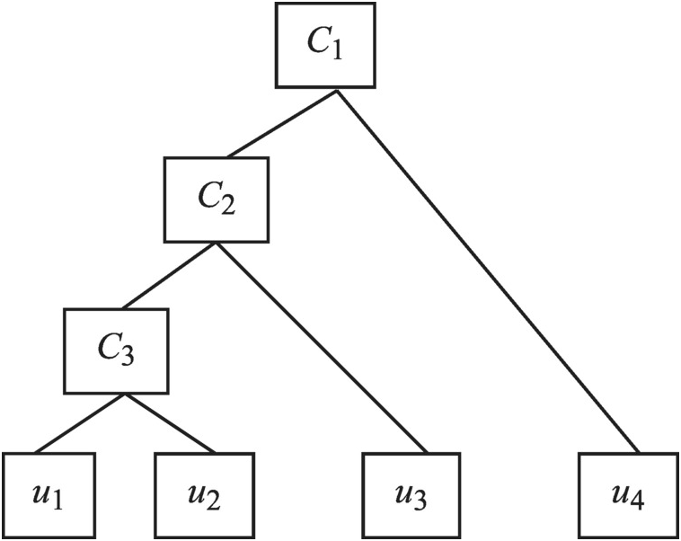
Figure 5.1 Four-dimensional FNAC structure.
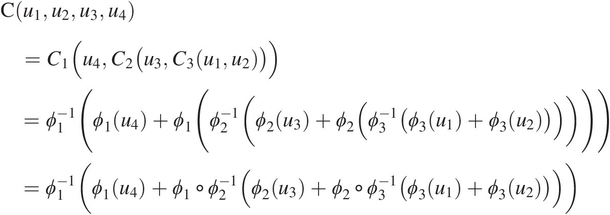
From Figure 5.1, it is seen that three bivariate copulas are needed to represent the dependence for the four-dimensional random variables through FNAC as follows. First, random variables u1u1 and u2u2 are coupled through copula C3C3. Second, random variable u3u3 is coupled with C3(u1, u2)C3u1u2 through copula C2C2. Third, random variable u4u4 is coupled with C2(u3, C3(u1, u2))C2u3C3u1u2 through copula C1C1. Hence, a four-dimensional copula requires three bivariate copulas C1, C2C1,C2, and C3C3, with generators ϕ1ϕ1, ϕ2ϕ2, and ϕ3ϕ3 and may be written as follows:
 (5.1)
(5.1)where ○ represents the composition of functions.
Similarly, the FNAC for d-dimensional random variables (e.g., Joe, 1997; Embrechts et al., 2003; Whelan, 2004; Nelsen, 2006) may be generated as follows:
 (5.2)
(5.2)It is worth noting that Equation (4.1) in Chapter 4, i.e., the exchangeable symmetric Archimedean copula, is a special case of Equation (5.2) if ϕ(θ1) = ϕ2(θ2) = … = ϕd − 1(θd − 1) = ϕ(θ), θ1 = θ2 = … = θd − 1ϕθ1=ϕ2θ2=…=ϕd−1θd−1=ϕθ,θ1=θ2=…=θd−1. For the d-dimensional FNAC, the bivariate margins themselves are also Archimedean copulas that allow for free specification of d – 1 copulas with the remaining identified implicitly through FNAC (Whelan, 2004; Berg and Aas, 2007). Using Equation (5.1) (Figure 5.1) as an example, this statement may be expressed as follows: (i) there are three Archimedean copulas of free specification, i.e., C3C3 with parameter θ3θ3 for variables u1, u2u1,u2; C2C2 with parameter θ2θ2 for variables {u3, C3(u1, u2; θ3}{u3,C3(u1,u2;θ3}; and C1C1 with parameter θ1θ1 for variables {u4, C2(u3, C3(u1, u2; θ3); θ2}{u4,C2(u3,C3u1u2θ3;θ2}; (ii) pairs (u1, u3), (u2, u3)u1u3,u2u3 have copula C2C2 with parameter θ2θ2; and (iii) pairs (u1, u4), (u2, u4), (u3, u4)u1u4,u2u4,u3u4 have copula C3C3 with parameter θ1θ1. The decreasing degree of dependence for the increasing levels of nesting (i.e., θ1 ≤ θ2 ≤ … ≤ θd − 1θ1≤θ2≤…≤θd−1 with θ1θ1 and θd − 1θd−1 representing the parameters for the highest and lowest levels, respectively) is another technical condition for proper construction of the d-dimensional fully nested asymmetric Archimedean copula.
It should also be pointed out that the following conditions need to be satisfied for the nested generating functions:
ϕ1−1,ϕ2−1,…,ϕd−1−1
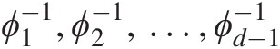 must satisfy the necessary conditions for being completely monotonic.
According to Embrechts et al. (2003), the coupling of functions wk=ϕk∘ϕk+1−1
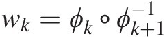 belongs to a class of functions ℒ∞∗
 defined as follows:
ℒ∞∗=ω:0∞→0∞ω0=0ω∞=∞−1k−1dkωtdt≥0k=12…∞ (5.3)
(5.3)


Based on Equation (5.2), the simplest three-dimensional FNAC (shown in Figure 5.2) can be written as follows:
 (5.4)
(5.4)
Figure 5.2 Three-dimensional FNAC structure.
In accordance with Equation (5.4), we outline here the derivation of five three-dimensional asymmetric Archimedean copulas that are commonly applied.
M3 (Joe, 1997):

Let t = C2(u1, u2)t=C2u1u2. Then we have C1u3t=−1θ1ln1−1−e−θ1u3(1−e−θ1t1−e−θ1
 (5.5)
(5.5)θ2 ≥ θ1 ∈ [0, ∞), τ12, τ13, τ23 ∈ [0, 1]θ2≥θ1∈0∞,τ12,τ13,τ23∈01 for positive dependent trivariate variables.
The M3 copula may be also called the asymmetric trivariate Frank copula.
We now use the following specific examples to illustrate these marginal distributions.
Example 5.1 Derive the M3 copula for θ1 = 2.0 and θ2 = 3.0θ1=2.0andθ2=3.0 by setting u3 = 0.6u3=0.6. Assuming u1~F1(x1) : X1~gamma(2, 4); u2~F2(x2) : X2~normal(1, 32); u3~F3(x3) : X3~EV1(10, 7)u1~F1x1:X1~gamma24;u2~F2x2:X2~normal132;u3~F3x3:X3~EV1107, and {X1, X2}X1X2 has a higher pairwise dependence.
Solution: With {X1, X2}X1X2 having higher pairwise dependence, we first couple X1and X2X1andX2 and build the copula function from the marginals as follows:


Since we already set u3 = 0.6u3=0.6, then we have x3≈9.388x3≈9.388 from the EV1 population.
Finally, we can write the fully nested copula using the M3 copula as follows:


Figure 5.3(a) plots the corresponding joint CDF for the derived M3 copula with u3 = 0.6u3=0.6. M4 (Joe, 1997):

Let t = C2(u1, u2)t=C2u1u2. Then we have C1u3t=u3−θ1+t−θ1−1−1θ1
 (5.6)
(5.6)θ2 ≥ θ1 ∈ [0, ∞), τ12, τ13, τ23 ∈ [0, 1]θ2≥θ1∈0∞,τ12,τ13,τ23∈01 for positive dependent trivariate variables. The M4 copula may also be called the trivariate asymmetric Clayton copula.

Figure 5.3 Joint CDF for derived FNACs: (a) M3 copula, (b) M4 copula, (c) M5 copula, (d) M6 copula, and (e) M12 copula.
Example 5.2 Derive the M4 copula using information given in Example 5.1.
Solution: In Example 5.1, we have θ1 = 2.0, θ2 = 3.0θ1=2.0,θ2=3.0 by setting u3 = 0.6u3=0.6. Thus, we have the following:


Figure 5.3(b) plots the corresponding joint CDF for the derived M4 copula with u3 = 0.6u3=0.6.
M5 (Joe, 1997):

Let t=C2u1u2,1−t=1−u1θ2+1−u2θ2−1−u1θ21−u2θ21θ2 . Then we have the following:
 (5.7)
(5.7)θ2 ≥ θ1 ∈ [1, ∞), τ12, τ13, τ23 ∈ [0, 1]θ2≥θ1∈1∞,τ12,τ13,τ23∈01. The M5 copula may also be called the trivariate asymmetric Joe copula.
Example 5.3 Derive M5 copula using the information given in Example 5.1.
Solution: In Example 5.1, we have θ1 = 2.0, θ2 = 3.0θ1=2.0,θ2=3.0 by setting u3 = 0.6u3=0.6. Thus we have the following:


Figure 5.3(c) plots the corresponding joint CDF for the derived M5 copula with u3 = 0.6u3=0.6.
M6 (Joe, 1997; Embrechts, 2003):
Let C2u1u2=e−−lnu1θ2+−lnu2θ21θ2,and

 (5.8)
(5.8)θ2 ≥ θ1 ∈ [1, ∞), τ12, τ13, τ23 ∈ [0, 1]θ2≥θ1∈1∞,τ12,τ13,τ23∈01 for positive dependent trivariate variables. The M6 copula may also be called the trivariate asymmetric Gumbel–Hougaard copula.
Example 5.4 Derive the M6 copula using the information given in Example 5.1.
Solution: In Example 5.1, we have θ1 = 2.0, θ2 = 3.0θ1=2.0,θ2=3.0 by setting u3 = 0.6u3=0.6. Thus we have the following:


Figure 5.3(d) plots the corresponding joint CDF for the derived M6 copula with u3 = 0.6u3=0.6.
M12 (Embrechts, 2003):

Let t=C2u1u2,1t−1=1u1−1θ2+1u2−1θ21θ2 . Then we have
 (5.9)
(5.9)
Example 5.5 Derive the M12 copula using the information given in Example 5.1.
Solution:


Figure 5.3(e) plots the joint CDF for the derived M12 copula with u3 = 0.6u3=0.6.
Solution: From Figure 5.1, we have the following:

C3C3 and u3u3 are coupled as copula C2(C3, u3)C2C3u3 with parameter θ2θ2, which can be written as follows:

Finally, C2C2 and u4u4 are defined as copula C1(C2, u4)C1C2u4 with parameter θ1θ1, which results in C1(C2, u4; θ1) = C(u1, u2, u3, u4; θ1, θ2, θ3)C1C2u4θ1=Cu1u2u3u4θ1θ2θ3 as follows:

In the same way as for the previous examples, for the four-dimensional random variables {Xi, i = 1, …, 4}Xii=1…4, the random variable XiXi may follow different marginal distributions as follows:


5.2.2 Partially Nested Archimedean Copulas (PNAC)
Originally, Joe (1997) proposed the structure of PNAC as an alternative approach for FNAC. PNAC may be considered a composite of EAC and FNAC (Berg and Aas, 2007).Similar to FNAC, PNAC also has d – 1 bivariate copulas that are partially exchangeable. As a simple example, Figure 5.4 illustrates the PNAC structure for four-dimensional random variables: (1) couple the two pairs (u1, u2)u1u2 and (u3, u4)u3u4 with copula C3C3 with parameter θ3θ3 and C2C2 with parameter θ2,θ2, respectively, at the first level; and (2) the third copula C1C1 with parameter θ1θ1 will be applied to couple C2C2 and C3C3 at the second level (Berg and Aas, 2007). Figure 5.4 also shows (1) exchangeability between u1u1 and u2u2, as well as between u3u3 and u4u4; and (2) four pairs (u1, u3), (u1, u4), (u2, u3)u1u3,u1u4,u2u3, and (u2, u4)u2u4 all have copula C1C1. Furthermore, the same constraints on parameters for FNAC are required to be satisfied for PNAC (Berg and Aas, 2007), i.e., (i) PNAC may be used to model the positively dependent variables, and (ii) the dependence decreases with the increase of nesting levels (i.e., the parameters of a higher level are smaller than those of a lower level).

Figure 5.4 Partially nested Archimedean construction.
Example 5.7 Using the bivariate Frank copula as the building block to derive a four-dimensional PNAC function for the structure given in Figure 5.4.
Solution: As shown in Figure 5.4, (u1, u2)u1u2 and (u3, u4)u3u4 can be represented through the Frank copula as follows:


Then C1C1 can be represented through C3, C2C3,C2 as follows:

with the parameters: 0 ≤ θ1 ≤ θ2, θ30≤θ1≤θ2,θ3.
In the same manner for FNAC, random variables {X1 : i = 1, 2, 3, 4}X1:i=1234 may follow different marginal distributions as ui = Fi(xi)ui=Fixi.
5.2.3 General Case
Originating in Joe (1997), the general nested Archimedean copula (GNAC) construction was further developed by Whelan (2004) and Savu and Trede (2006). Savu and Trede (2006) first introduced the notation for arbitrary nesting and the procedure for calculating the d-dimensional probability density function in general. To build a hierarchy of Archimedean copulas, they also applied the notation for the hierarchical Archimedean copula for GNAC. The main idea of the generally nested Archimedean construction is presented in this section (Berg and Aas, 2007).
For the GNAC with L levels, there are nlnl distinct objects (an object is either a copula or a variable) at each level l. At level l = 1l=1, variables u1, …, udu1,…,ud are grouped into n1n1 exchangeable multivariate Archimedean copulas. These copulas are, in turn, coupled with n2n2 copula at level l = 2l=2, and so on. Berg and Aas (2007) presented an example of a nine-dimensional copula to explain this structure (Figure 5.5).

Figure 5.5 Hierarchically nested Archimedean copula construction.
Following Figure 5.5, the nine-dimensional copula can be written as
At the first level, there are two two-dimensional EACs, i.e., C41(u1, u2)C41u1u2 with parameter θ41θ41 and C42(u8, u9)C42u8u9 with parameter θ42θ42. There are one three-dimensional and one two-dimensional EACs at the second level, i.e., C31(C41, u3, u4)C31C41u3u4 with parameter θ31θ31 and C32(u7, C42)C32u7C42 with parameter θ32θ32. At the third level, there is only one copula, C21(C31, u5, u6)C21C31u5u6 with parameter θ21θ21. At the top (fourth) level, the copula C11C11, with parameter θ11θ11, is applied to model the dependence between C21C21 and C32C32.
To ensure that GNAC is a valid Archimedean copula, there are a number of conditions that need to be satisfied (Savu and Trede, 2006; Berg and Aas, 2007):
a. The number of copulas must decrease with the increasing level of nesting. The top level may contain only one copula, and the inverse of the generating functions (ϕ−1ϕ−1) must be completely monotonic.
b. The dependence of GNAC must decrease with the increasing level of nesting. For example, in Figure 5.5, parameters must be stratified following the condition θ41 ≥ θ32 ≥ θ21 ≥ θ11θ41≥θ32≥θ21≥θ11 and θ42 ≥ θ32 ≥ θ11θ42≥θ32≥θ11. However, when mixing copula generators that belong to different Archimedean copula families, this requirement might not be sufficient. Two Archimedean copulas from different families (i.e., Fam1 and Fam2) can only be nested if the derivative of the product ϕ1∘ϕ2−1
 is completely monotonic. Joe (1997) presented details about copula families that can be mixed and explored structures where all the generators are from the same family are explored, and the other structures are still not fully explored.

5.2.4 Parameter Estimation for Nested Copulas
For NAC with an explicit density expression, the maximum likelihood estimation method is commonly applied to estimate the copula parameters; however, the NAC density function may not be straightforwardly derived. Savu and Trede (2006) proposed a recursive approach to derive the density function for general NAC. With this approach, the number of computational steps for evaluating the density increases rapidly with the copula complexity, and parameter estimation becomes very time consuming in higher dimensions (Savu and Trede, 2006; Berg and Aas, 2007).
The density function of NAC can be derived using the chain rule as discussed by Savu and Trede (2006). We will use the following examples to illustrate the general procedure on how to apply the chain rule. Furthermore, we derive the density functions for the M3, M4, M5, M6, and M12 copulas (Joe, 1997) in the appendix as specific examples.
Example 5.8 Derive the density function for three-dimensional FNAC (Equation (5.4) corresponding to Figure 5.2).
Solution: Equation (5.4) may be rewritten as follows:
C(u1, u2, u3) = C1(C2(u1, u2), u3)Cu1u2u3=C1C2u1u2u3 and its density, i.e., c(u1, u2, u3)cu1u2u3, may be derived as follows:

Finally, we have the following:

Example 5.9 Derive the density function for four-dimensional FNAC (i.e., Equation (5.1) corresponding to Figure 5.1).
Solution: Following Equation (5.1) and Figure 5.1, we have the following:
C(u1, u2, u3, u4) = C1(u4, C2) = C1(u4, C2(u3, C3(u1, u2)))Cu1u2u3u4=C1u4C2=C1u4C2u3C3u1u2 and its density c(u1, u2, u3, u4)cu1u2u3u4 may be derived as follows:

Finally, we have the following:

Example 5.10 Derive the density function for the copula function represented by Figure 5.4.
Solution: According to Figure 5.4, we have the following: C(u1, u2, u3, u4) = C1(C3(u1, u2), C2(u3, u4)).Cu1u2u3u4=C1C3u1u2C2u3u4. Then its density function c(u1, u2, u3, u4)cu1u2u3u4 may be expressed as follows:


Finally, we have the following:

With the copula density function derived, we can then apply MLE to estimate parameters simultaneously with the constraints of parameters at a lower level being larger than those at a higher level. However, the copula parameters may also be estimated sequentially with the use of MLE as follows:
i. Estimate the copula parameter at the lowest level.
ii. Estimate the copula parameter for the second-lowest level by fixing the parameters estimated for the lowest level.
iii. Repeat the preceding steps until we reach the top level of the NAC structure.
5.2.5 Simulation for Nested Copulas
In the previous chapters, we have shown that EAC may be simulated with several methods, such as Laplace transform (LT) and CPI Rosenblatt’s transform, and through its unique generating function ϕϕ with a simple algorithm. Frees and Valdez (1998) showed how to use the LT method to simulate NACs for the generators taken from either the Gumbel– Hougaard or the Clayton copula family. However, Berg and Aas (2007) have pointed out that the LT method is limited to the copulas such that we can find a distribution that equals the LT of the inverse generating function and from which we can easily sample. In most cases, the LT method needs to obtain the d – 1 first derivatives of the copula function, which usually yield extremely complex expressions under higher-order derivatives. The limitation of LT method may cause the simulation to become inefficient for high dimensions (Berg and Aas, 2007).
Compared to the LT method, the CPI Rosenblatt transform method is more universal and will be introduced to simulate from NAC. Let X = {X1, X2, …, Xd}X=X1X2…Xd be a d-dimensional random vector with marginal distributions F(xi)Fxi and conditional distributions F(xi| x1, …, xi − 1), i = 1, …, dFxix1…xi−1,i=1,…,d. The CPI Rosenblatt’s transform of X is defined as T(X) = {T(X1), …, T(Xd)}TX=TX1…TXd:
With the use of CPI method, random variables are simulated with the following procedure:
i. Generate W = {w1, w2, …, wd}W=w1w2…wd independent random variables following the uniform distribution [0, 1].
ii. Set x1 = w1x1=w1.
iii. Set w2 = T(X2) = F2 ∣ 1(x2| x1)w2=TX2=F2∣1x2x1 to obtain x2=F2∣1−1w2x1.
iv. Set w3 = T(X3) = F3 ∣ 1, 2(w3| x1, x2)w3=TX3=F3∣1,2w3x1x2 to obtain x3=F3∣1,2−1w3x1x2
 .
.
…
Set wd = T(Xd) = Fd ∣ 1, 2, …d − 1(wd| x1, x2, …, xd)wd=TXd=Fd∣1,2,…d−1wdx1x2…xd.


Example 5.11 Assuming the pseudo-observations given in Table 5.1 may be modeled with the M6 copula, (1) estimate the copula parameters both simultaneously and sequentially using MLE; and (2) simulate the random variables with a sample size of 50.
Table 5.1. Trivariate pseudo-observations.
| u1u1 | u2u2 | u3u3 | |
|---|---|---|---|
| 1 | 0.241 | 0.138 | 0.103 |
| 2 | 0.241 | 0.172 | 0.172 |
| 3 | 0.241 | 0.241 | 0.276 |
| 4 | 0.241 | 0.586 | 0.655 |
| 5 | 0.793 | 0.828 | 0.897 |
| 6 | 0.483 | 0.345 | 0.379 |
| 7 | 0.931 | 0.914 | 0.621 |
| 8 | 0.724 | 0.759 | 0.724 |
| 9 | 0.414 | 0.621 | 0.586 |
| 10 | 0.759 | 0.414 | 0.310 |
| 11 | 0.862 | 0.793 | 0.793 |
| 12 | 0.655 | 0.517 | 0.448 |
| 13 | 0.414 | 0.379 | 0.552 |
| 14 | 0.569 | 0.448 | 0.414 |
| 15 | 0.569 | 0.690 | 0.690 |
| 16 | 0.414 | 0.310 | 0.241 |
| 17 | 0.241 | 0.552 | 0.862 |
| 18 | 0.069 | 0.035 | 0.035 |
| 19 | 0.241 | 0.276 | 0.345 |
| 20 | 0.069 | 0.069 | 0.069 |
| 21 | 0.897 | 0.914 | 0.931 |
| 22 | 0.655 | 0.655 | 0.483 |
| 23 | 0.069 | 0.103 | 0.138 |
| 24 | 0.241 | 0.207 | 0.207 |
| 25 | 0.655 | 0.724 | 0.759 |
| 26 | 0.517 | 0.483 | 0.517 |
| 27 | 0.828 | 0.862 | 0.828 |
| 28 | 0.966 | 0.966 | 0.966 |
Solution: Estimate the copula parameters.
To estimate the parameters for the fitted M6 copula, we use Figure 5.2 as the FNAC scheme.
Estimate the copula parameters simultaneously.
To estimate the copula parameters simultaneously, the copula density function (i.e., Equation (M6–3) in the appendix) is applied to write the log-likelihood function as follows:
logL=∑1u1u2u3−lnu1θ2−1−lnu2θ2−1−lnu3θ3−1e−w1θ1(G2θ1θ2−2w3θ1−3+2θ1−2w2θ1−2+θ2−θ1Gθ1θ2−2w2θ1−2+θ1−12θ1−1G2θ1θ2−2w1θ1−3+θ1−1G2θ1θ2−2w2θ1−3+θ1−1θ2−θ1Gθ1θ2−2w1θ1−2)where G =−lnu1θ2+−lnu2θ2;w=−lnu3θ1+[−lnu1θ2+−lnu2)θ1θ1θ2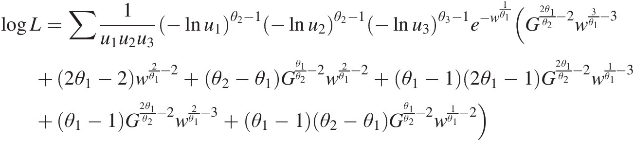
 .
.
The parameter constraint is given as 1 ≤ θ1 ≤ θ21≤θ1≤θ2, where θ2θ2 corresponds to the parameters for the first level.
Maximizing the log-likelihood function numerically (e.g., using genetic algorithm ga function in MATLAB), the parameters are estimated as follows:
θ2 = 4.4158; θ1 = 3.3532θ2=4.4158;θ1=3.3532.
It is worth noting that to properly estimate the parameters simultaneously, the linear constraint needs to be applied with vector A = [–1,1] B = 0, which represents –θ2 + θ1 ≤ 0–θ2+θ1≤0.
Estimate the copula parameters sequentially.
To estimate the copula parameters sequentially, the density function for the bivariate Gumbel–Hougaard copula is applied (Chapter 4).
Step 1: Maximizing the log-likelihood function for (u1, u2)u1u2, we have θ2 = 4.4682θ2=4.4682.
Step 2: Compute C(u1, u2; θ2 = 4.4682C(u1,u2;θ2=4.4682) and estimate the parameter for
(u3, C(u1, u2; θ2 = 4.4682))u3Cu1u2θ2=4.4682. Again using MLE, we have θ1 = 3.2088θ1=3.2088. It is worth noting that to estimate the parameter (i.e., the Gumbel–Hougaard copula) for the top level, the lower and upper bounds are [1, θ2]1θ2.
Finally, for both simultaneous and sequential estimation, the parameters estimated are coded as follows:
param = [param(1), param(2)] = [θ2, θ1]param=param1param2=θ2θ1; param(1) and param(2) represents bottom and top levels, respectively.
Simulation from the fitted M6 copula.
As discussed previously, the random variates are simulated using the CPI Rosenblatt transform, as shown in Figure 5.6(a).


In addition, we have discussed previously that [u1, u3]u1u3 and [u2, u3]u2u3 may be modeled with the Gumbel–Hougaard copula with parameter θ1θ1. Figure 5.6(b) compares the simulation as well as the box plot of simulated and sample Kendall’s tau (100 simulations with a sample size of 28).


Figure 5.6 (a) Comparison of pseudo-observations with those simulated from M6 copula; (b) simulation comparison from the Gumbel–Hougaard copula with parameter θ1θ1 for (u1, u3), (u2, u3)u1u3,u2u3 directly; (c) comparison of sample Kendall’s tau with simulated Kendall’s tau from Gumbel–Hougaard copula with parameter θ = 2.8816θ=2.8816.
Example 5.12 Assuming the Gumbel–Hougaard copula may be applied as a biviarate building block, and using the scheme shown in Figure 5.4 and the pseudo-observations listed in Table 5.2, (1) estimate the copula parameters; and (2) simulate random variates with fitted copula for a sample size of 100.
Table 5.2. Pseudo-observations for Example 5.12.
| u1u1 | u2u2 | u3u3 | u4u4 | |
|---|---|---|---|---|
| 1 | 0.194 | 0.338 | 0.421 | 0.545 |
| 2 | 0.819 | 0.901 | 0.743 | 0.705 |
| 3 | 0.614 | 0.639 | 0.615 | 0.662 |
| 4 | 0.235 | 0.208 | 0.298 | 0.292 |
| 5 | 0.792 | 0.755 | 0.865 | 0.894 |
| 6 | 0.433 | 0.517 | 0.559 | 0.480 |
| 7 | 0.130 | 0.197 | 0.095 | 0.087 |
| 8 | 0.570 | 0.583 | 0.802 | 0.680 |
| 9 | 0.128 | 0.274 | 0.256 | 0.137 |
| 10 | 0.218 | 0.116 | 0.262 | 0.481 |
| 11 | 0.468 | 0.367 | 0.367 | 0.439 |
| 12 | 0.490 | 0.434 | 0.391 | 0.515 |
| 13 | 0.194 | 0.083 | 0.019 | 0.042 |
| 14 | 0.120 | 0.227 | 0.178 | 0.289 |
| 15 | 0.676 | 0.601 | 0.759 | 0.673 |
| 16 | 0.990 | 0.990 | 0.991 | 0.993 |
| 17 | 0.657 | 0.777 | 0.942 | 0.950 |
| 18 | 0.226 | 0.174 | 0.284 | 0.134 |
| 19 | 0.828 | 0.857 | 0.836 | 0.916 |
| 20 | 0.373 | 0.367 | 0.151 | 0.249 |
| 21 | 0.698 | 0.656 | 0.727 | 0.584 |
| 22 | 0.645 | 0.738 | 0.641 | 0.787 |
| 23 | 0.025 | 0.051 | 0.034 | 0.199 |
| 24 | 0.298 | 0.300 | 0.470 | 0.394 |
| 25 | 0.906 | 0.936 | 0.955 | 0.950 |
| 26 | 0.658 | 0.476 | 0.556 | 0.647 |
| 27 | 0.302 | 0.158 | 0.224 | 0.105 |
| 28 | 0.581 | 0.393 | 0.733 | 0.779 |
| 29 | 0.371 | 0.433 | 0.179 | 0.145 |
| 30 | 0.169 | 0.537 | 0.213 | 0.344 |
| 31 | 0.041 | 0.083 | 0.009 | 0.059 |
| 32 | 0.982 | 0.978 | 0.928 | 0.935 |
| 33 | 0.585 | 0.162 | 0.326 | 0.312 |
| 34 | 0.618 | 0.753 | 0.661 | 0.633 |
| 35 | 0.280 | 0.622 | 0.400 | 0.574 |
| 36 | 0.902 | 0.969 | 0.879 | 0.904 |
| 37 | 0.440 | 0.648 | 0.587 | 0.811 |
| 38 | 0.243 | 0.147 | 0.281 | 0.524 |
| 39 | 0.044 | 0.081 | 0.177 | 0.052 |
| 40 | 0.122 | 0.149 | 0.229 | 0.180 |
| 41 | 0.497 | 0.645 | 0.528 | 0.545 |
| 42 | 0.701 | 0.644 | 0.745 | 0.599 |
| 43 | 0.323 | 0.538 | 0.806 | 0.796 |
| 44 | 0.013 | 0.044 | 0.063 | 0.041 |
| 45 | 0.651 | 0.721 | 0.774 | 0.646 |
| 46 | 0.190 | 0.298 | 0.773 | 0.841 |
| 47 | 0.520 | 0.772 | 0.636 | 0.542 |
| 48 | 0.926 | 0.943 | 0.900 | 0.812 |
| 49 | 0.468 | 0.447 | 0.518 | 0.633 |
| 50 | 0.868 | 0.894 | 0.893 | 0.905 |
| 51 | 0.422 | 0.710 | 0.727 | 0.560 |
| 52 | 0.888 | 0.835 | 0.868 | 0.823 |
| 53 | 0.372 | 0.590 | 0.734 | 0.792 |
| 54 | 0.132 | 0.116 | 0.095 | 0.041 |
| 55 | 0.429 | 0.288 | 0.219 | 0.125 |
| 56 | 0.390 | 0.366 | 0.375 | 0.172 |
| 57 | 0.983 | 0.986 | 0.991 | 0.990 |
| 58 | 0.980 | 0.988 | 0.976 | 0.974 |
| 59 | 0.308 | 0.318 | 0.147 | 0.193 |
| 60 | 0.932 | 0.913 | 0.943 | 0.933 |
Solution:
1. Estimate the copula parameters.
According to Figure 5.4, let us use θ12, θ34θ12,θ34 to represent the copula parameters of [u1, u2], [u3, u4]u1u2,u3u4 at the bottom level and θθ to represent the copula parameter at the top level.
Estimate the parameters simultaneously.
Given the Gumbel–Hougaard copula as a bivariate building block, the copula density function for the four-dimensional PNAC Gumbel–Hougaard copula may be derived based on the chain rule following the procedure given in Example 5.10. With the parameter constraints 1 ≤ θ ≤ θ12, θ341≤θ≤θ12,θ34, i.e.,
θ−θ12≤0θ−θ34≤0
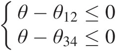 , the inequality vector is then given as A=−1,0,10,−1,1,B=00
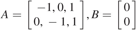 , with the parameter set as param = [θ12, θ34, θ]param=θ12θ34θ.
The parameters can be estimated numerically by maximizing the log-likelihood function with the preceding linear constraint as follows:
θ12 = 3.6949, θ34 = 4.5035, θ = 2.8816θ12=3.6949,θ34=4.5035,θ=2.8816.
Estimate the parameters sequentially.
With the same estimation procedures shown in Example 5.11:
The parameter for (u1, u2)u1u2 is estimated as θ12 = 3.8545θ12=3.8545.
The parameter for (u3, u4)u3u4 is estimated as θ34 = 4.3949θ34=4.3949.
The parameter for {C3(u1, u2; θ12), C2(u3, u4; θ34)}C3u1u2θ12C2u3u4θ34 is estimated by fixing θ12, θ34θ12,θ34 as θ = 3.3297θ=3.3297.
2. Simulate random variates.
Using the CPI Rosenblatt transform, Figure 5.7(a) compares the pseudo-observations in Table 5.2 with those simulated from the fitted PNAC Gumbel–Hougaard copula function.


Figure 5.7 (a) Comparison of pseudo-observations with those simulated with the parameters estimated simultaneously (θ12 = 3.6949, θ34 = 4.5035, θ = 2.8816θ12=3.6949,θ34=4.5035,θ=2.8816); (b) comparison of observed variables with simulated variables with θ = 2.8816θ=2.8816; (c) comparison of sample Kendall’s tau with the simulated Kendall’s taus.
As discussed previously for the PNAC structure, we know (u1, u3), (u1, u4), (u2, u3), (u2, u4)u1u3,u1u4,u2u3,u2u4 should have the same joint distribution that may be modeled using the Gumbel–Hougaard copula with parameter at the top level, i.e., θ = 2.8816θ=2.8816 with the comparison of simulated random variable and Kendall’s tau as shown in Figure 5.7(b) and 5.7(c). Figure 5.7(b) and 5.7(c) indicates that the preceding four pairs may be modeled using the same Gumbel–Hougaard copula.
5.3 Pair-Copula Construction (PCC)
PCCs are also hierarchical in nature. Compared to EAC and NAC, a large improvement is made in PCCs that allows for the free specification of dd−12 copulas. The modeling scheme of PCCs is based on the decomposition of a multivariate density function. The d-dimensional probability density function may be decomposed to dd−12
 bivariate density functions, where the first d − 1d−1 density functions are unconditional and the rest are conditional (Berg and Aas, 2007). First proposed by Joe (1997), there are two main types of PCCs, canonical (C)-vines and D-vines, in the literature (e.g., Bedford and Cooke, 2001, 2002; Kurowicka and Cooke, 2004, 2006; Aas et al., 2009).
5.3.1 Principle of Pair-Copula Decomposition of General Multivariate Distribution
Following Aas et al. (2009), we introduce the pair-copula decomposition of general multivariate distributions.
Let X = (X1, X2, …, Xd)X=X1X2…Xd be a vector of random variables with a joint density function f(x1, …, xd)fx1…xd. According to the conditional probability theory, the joint density function can be defined as follows:
In Chapters 3 and 4, the multivariate distribution F with marginals F1(x1), …, Fd(xd)F1x1,…,Fdxd is defined using Sklar’s theorem as follows:
 (5.13)
where ui = Fi(xi)ui=Fixi; Fi−1ui is the inverse distribution of marginal Fi(xi)Fixi.
Then, for an absolutely continuous F with strictly increasing, continuous marginal probability densities f1(x1), …, fd(xd)f1x1,…,fdxd, applying ∂d∂x1…∂xd to Equation (5.13), we have
 (5.14a)
 (5.14b)
where c1, 2, …, d(⋅)c1,2,…,d⋅ stands for the d-dimensional copula density function.
In the bivariate case, Equation (5.14b) can be simplified to
where c12(⋅)c12⋅ is the appropriate pair-copula density.
Using the conditional probability in Equation (5.12), the conditional probability density function can be easily written as
 (5.16)
Likewise, we have
Similarly, in the trivariate case, we can obtain the conditional probability density function:
 (5.18)
According to the definition of conditional copula, we have
 (5.19)
Thus,
 (5.20)
Alternatively, f(x1| x2, x3)fx1x2x3 may be also written as follows:
Equations (5.20) and (5.21) can be further decomposed as follows:
From the expression of the appropriate pair-copula, a conditional marginal density function can be expressed in a general form as follows:
where v is a d-dimensional vector; vjvj is one arbitrarily chosen component of v; and v−jv−j denotes the v vector except vjvj, i.e., v−j = v\vjv−j=v\vj.
Under appropriate conditions, a multivariate probability density function may be expressed through the product of pair-copulas, acting on several different conditional probability distributions (Aas et al., 2009).
Joe (1997) showed a conditional marginal distribution for the appropriate pair-copula for every j as
 (5.24)
where Cx, vj ∣ v−jCx,vj∣v−j is a bivariate copula function with the conditional marginals. For the special case where v is univariate, Equation (5.24) can be rewritten as follows:
 (5.25)
In Equation (5.25), when xx and vv are copula random variables (i.e., the margins following the uniform [0,1] as f(x) = f(v) = 1, FX(x) = x, FV(v) = vfx=fv=1,FXx=x,FVv=v), Equation (5.25) can be rewritten as follows:
 (5.26)
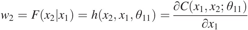
where the second variable of h(⋅)h⋅ function represents the conditional variable, and ΘΘ denotes the set of copula parameters to model the joint distribution function of xx and vv. Letting u = xu=x, Equation (5.26) is essentially the conditional copula function of C(u| V = v; Θ)CuV=vΘ.
Solution: As seen in the previous chapters, the bivariate Gumbel–Hougaard copula can be written as follows:

Then the hh function, i.e., h(u1, u2, θ)hu1u2θ, can be expressed as follows:

5.3.2 Vines
High-dimensional distributions have a significant number of possible pair-copula constructions. The regular vine, introduced by Bedford and Cooke (2001, 2002), is used to organize the general structure and embrace a large number of possible pair-copula decompositions. Two special types of regular vines, the C-vine and the D-vine (Kurowicka and Cooke, 2004), are given in the form of a nested set of trees and are used to decompose the multivariate density function. Figure 5.8 shows one sample specification corresponding to a five-dimensional D-vine that can be explained with Table 5.3.

Figure 5.8 A D-vine with five variables, four trees, and 10 edges.
Table 5.3. Five-dimensional D-vine.
| Tree TjTj | Nodes | Edges |
|---|---|---|
| T1T1 | 1, 2, 3, 4, 5 | 12, 23, 34, 45 |
| T2T2 | 12, 23, 34, 45 | 13|2, 24|3, 35|4 |
| T3T3 | 13|2, 24|3, 35|4 | 14|23, 25|34 |
| T4T4 | 14|23, 25|34 | 15|234 |
In Figure 5.8 and Table 5.3, each edge represents a pair-copula density, and the edge label corresponds to the subscript of the pair-copula density. For example, 14|23 corresponds to the copula density c14 ∣ 23(C13 ∣ 2, C24 ∣ 3)c14∣23C13∣2C24∣3. The entire decomposition is defined by dd−12=55−12=10 edges as well as the density functions of random variables.
The density function of random variable X = {X1, X2, …, Xd}X=X1X2…Xd with a D-vine copula can be written as
 (5.27)
where index jj identifies the trees, and ii identifies the edges in each tree.
A sample of C-vine with five variables is given in Figure 5.9. The meanings of symbols are the same as in Figure 5.8. We can see that each tree TjTj has a unique node connecting to d − jd−j edges in tree TjTj. For example, node 1 of tree T1T1 is connected to nodes 2, 3, 4, and 5 and forms the edges 12, 13, 14, and 15. Similarly, node 12 of T2T2 is connected to nodes 13, 14, and 15 and forms the edges 23|1, 24|1 and 25|1.

Figure 5.9 A C-vine with five variables, four trees, and 10 edges.
In general, the d-dimensional density function corresponding to a C-vine is defined as
 (5.28)
Looking at Figures 5.8 and 5.9, it is seen that the D-vine is more flexible than the C-vine. However, the C-vine might be advantageous if a particular variable is known to be the key variable governing interactions among the variables. In such a situation, one may decide to locate this variable at the root of the C-vine.
Following Aas et al. (2009), we present several typical pair-copulas.
Three Variables
For three-dimensional variables, there should be a total of six different pair-copula decompositions, including three D-vines and three C-vines. However, for three-dimensional variables, the D-Vine and C-vine are exactly the same, i.e., there are three different decompositions whose structures are both canonical vine and D-vine, as shown in Figure 5.10.

Figure 5.10 Decomposition schemes for three-dimensional variables using vines.
According to the decomposition schemes in Figure 5.10 and using Figure 5.10(a) as an example, the probability density function for both C-vine and D-vine structures can be written for three-dimensional random variables as
 (5.29)
where f1, f2, f3f1,f2,f3 and F1, F2, F3F1,F2,F3 represent the univariate PDF and CDF for variables x1, x2, x3x1,x2,x3, respectively.
Four Variables
For four-dimensional variables, we can construct a total of 24 different pair-copula decompositions, including 12 D-vines and 12 C-vines, as shown in Figure 5.11 (examples for one D-vine and one C-vine construction). Following the scheme, one may easily construct the rest D-vine and C-vine structures for four-dimensional variables.

Figure 5.11 Vines for four-dimensional variables: (a) D-vine; (b) C-vine).
According to Figure 5.11(a), the four-dimensional D-vine structure can be expressed as
 (5.30)
and according to Figure 5.11(b), the four-dimensional C-vine structure can be expressed as follows:
 (5.31)
Five Variables
For five-dimensional variables, there are 240 different possible pair-copula decompositions, including 60 C-vines (Figure 5.8, for example), 60 D-vines (Figure 5.9 is an example), and 120 other regular vine decompositions (Aas et al., 2009; shown in Figure 5.12 with two examples)


Figure 5.12 Two regular-vine examples for five-dimensional variables.
According to Figure 5.8, the general expression for the five-dimensional D-vine structure can be given as follows:
 (5.32)
According to Figure 5.9, the general expression for the five-dimensional C-vine structure can be given as
 (5.33)
According to Figure 5.12(a), the density function for a five-dimensional regular vine structure can be expressed as follows:
 (5.34a)
According to Figure 5.12(b), the density function for the five-dimensional regular vine can be expressed as follows:
 (5.34b)
d-Dimensional Variables
For a d-dimensional D-vine, Aas et al. (2009) concluded that there are d!d! possible ways of ordering the variables in tree T1T1. But only d ! /2d!/2 are different trees on the first level. Given such a tree T1T1, trees T1, T2, …, Td − 1T1,T2,…,Td−1 are completely determined. This implies that the number of distinct D-vines on d nodes is given by d ! /2d!/2. For a d-dimensional C-vine, there are also d ! /2d!/2 distinctive vine structures.
5.3.3 Conditional Independence and the Pair-Copula Decomposition
First, let us consider the three-dimensional case in Equation (5.29). If X1X1 and X3X3 are independent, conditioned on random variable X2X2, i.e., c13 ∣ 2(F1 ∣ 2(x1| x2), F3 ∣ 2(x3| x2)) = 1c13∣2F1∣2x1x2F3∣2x3x2=1, the density function in Equation (5.29) can be simplified as
Equation (5.35) indicates that the number of levels reduces to one with the assumption of conditional independence imposed for the three-dimensional variable.
Similarly, if X and Y are independent conditioned on any vector v, we have the following:
5.3.4 Simulation from Vine Copulas
As discussed previously in Section 5.2.5, the CPI Rosenblatt transformation is commonly applied for the simulation (or sampling) from vine copulas. The conditional probability of the jth variable conditioned on the previous j–1 variables, i.e., F(xj| x1, …, xj − 1)Fxjx1…xj−1, can be written using Equations (5.37) and (5.38) for C-vine and D-vine copulas, respectively, as follows.
For the C-vine copula, the conditional probability is
 (5.37)
For the D-vine copula structure, we use
 (5.38)
Here, we give the simulation procedure of the C-vine and D-vine copulas (Aas et al., 2009). In these algorithms, we first define that x = {x1…, xd}x=x1…xd are pseudo-observations (i.e., the maringal CDF: copula variables); we also define the parameters as T1 : θ11, …, θ1(d − 1)T1:θ11,…,θ1d−1, T2 : θ21, …, θ2(d − 2)T2:θ21,…,θ2d−2,…, Td − 1 : θ(d − 1)1Td−1:θd−11.
Simulation from a C-Vine Copula
The procedure for sampling from a C-vine copula can be described as algorithm 1 in Aas et al. (2009). This algorithm applies the margins (i.e., marginal CDF) as variable xx and variable 1 as the center variable. In other words, the algorithm simulates the pseudorandom variables rather than the random variables in a real domain. Algorithm 1 involves the following steps:
i. Generate d independent random numbers W = {w1, …, wd}W=w1…wd from uniform [0, 1] distribution. And we have x1 = u1 = w1x1=u1=w1 and wi = F(xi| x1, …, xi − 1), i = 2, .., dwi=Fxix1…xi−1,i=2,…,d.
ii. Simulate x2 = u2x2=u2 from u1u1 and w2w2 as x2 = u2 = h−1(w2, u1; θ11)x2=u2=h−1w2u1θ11.
iii. Simulate x3 = u3x3=u3 from u1, u2u1,u2 and w3w3, where w3 = C(u3| u1, u2)w3=Cu3u1u2 as follows:
Simulating C(u3| u1)Cu3u1:
w3=Cu3u1u2=∂C2,3∣1Cu3u1θ12Cu2u1θ11θ21∂Cu2u1=hC3∣1C2∣1θ21
C3 ∣ 1(u3| u1; θ12) = h−1(w3, C2 ∣ 1; θ21) = h−1(w3, w2; θ21)C3∣1u3u1θ12=h−1w3C2∣1θ21=h−1w3w2θ21
Simulating u3u3 using C3 ∣ 1C3∣1, which we just simulated, as follows:
u3 = h−1(C3 ∣ 1, u1; θ12)u3=h−1C3∣1u1θ12
iv. Simulate x4 = u4x4=u4 from u1, u2, u3,u1,u2,u3, and w4w4 with the following procedures:
Simulating C(u4| u1, u2)Cu4u1u2:
w4=Cu4u1u2u3θ31=∂C34∣12Cu4u1u2θ22Cu3u1u2θ21θ31∂Cu3u1u2θ21=∂C34∣12Cu4u1u2θ22w3θ31∂w3C4∣12u4u1u2=h−1w4w3θ31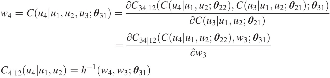
Simulating u4u4 using u1u1 and C2 ∣ 1 = w2C2∣1=w2 as follows:
C4∣12=∂C2,4∣1C4∣1C2∣1θ22∂C2∣1=∂C2,4∣1C4∣1w2θ22∂w2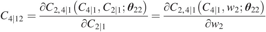
…
C4 ∣ 1 = h−1(h−1(w4, w3; θ31), w2; θ22) ⇒ u4 = h−1(C4 ∣ 1, u1; θ13)C4∣1=h−1h−1w4w3θ31w2θ22⇒u4=h−1C4∣1u1θ13


Carry on the logic for simulation until we reach the dimension d. And one may refer to Aas et al. (2009) for the exact algorithm.
Simulating the Random Variables for a D-Vine Copula
Algorithm 2 in Aas et al. (2009) provided the simulation procedure for the D-vine copula. As stated in Aas et al. (2009), algorithm 2 is less efficient than that for the C-vine copula. To simulate a d-dimensional D-vine copula, we will need to compute (d − 2)2d−22 conditional copulas, while we only need to compute(d − 2)(d − 1)/2d−2d−1/2 for a C-vine. Again, as with algorithm 1, algorithm 2 simulates the pseudorandom variables and includes the following steps:
i. Generate d-independent random numbers W = {w1, …, wd}W=w1…wd from uniform [0, 1] distribution. And we have x1 = u1 = w1x1=u1=w1 and wi = F(xi| x1, …, xi − 1), i = 2, .., dwi=Fxix1…xi−1,i=2,…,d;
ii. Simulate x2 = u2x2=u2 from u1u1 and w2w2 as x2 = u2 = h−1(w2, u1; θ11)x2=u2=h−1w2u1θ11.
iii. Simulate x3 = u3x3=u3 from u1, u2u1,u2 and w3w3 where w3 = C(u3| u1, u2)w3=Cu3u1u2 as follows:
Compute the conditional copula C1∣2=∂C12u1u2θ11∂u2
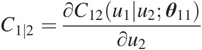
Simulate C(u3| u2)Cu3u2:
w3=Cu3u1u2=∂C1,3∣2Cu3u2θ12Cu1u2θ11θ21∂Cu1u2=hC3∣2C1∣2θ21
C3 ∣ 2(u3| u2; θ12) = h−1(w3, C1 ∣ 2; θ21) = h−1(w3, C1 ∣ 2; θ21)C3∣2u3u2θ12=h−1w3C1∣2θ21=h−1w3C1∣2θ21
Simulate u3u3 using C3 ∣ 1C3∣2, which we just simulated, as follows:
u3 = h−1(C3 ∣ 2, u2; θ12)u3=h−1C3∣2u2θ12
iv. Simulate x4 = u4x4=u4 from u1, u2, u3,u1,u2,u3, and w4w4 with the following procedures:
Compute the conditional copula C1 ∣ 23C1∣23:
C1∣23=∂C13∣2C1∣2C3∣2θ21∂C3∣2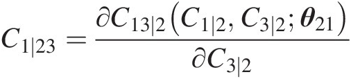
Simulate C(u4| u2, u3)Cu4u2u3:
w4=Cu4u1u2u3θ31=∂C14∣23Cu4u2u3θ22Cu1u2u3θ21θ31∂Cu1u2u3θ21=∂C14∣23Cu4u2u3θ22C1∣23θ31∂C1∣23C4∣23u4u2u3=h−1w4C1∣23θ31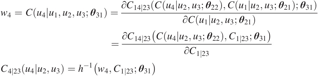
Compute C2 ∣ 3C2∣3:
C2∣3=∂C23u2u3θ12∂u3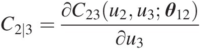
Simulate u4u4 using u3u3 and C2 ∣ 3C2∣3 as follows:
C4∣23=∂C2,4∣3C4∣3C2∣3θ22∂C2∣3⇒C4∣3=h−1C4∣23C2∣3θ22⇒u4=h−1C4∣3u3θ13…


Carry on the computation until we reach the d-dimension using Equation (5.38). Refer to Aas et al. (2009) for the exact algorithm.
Example 5.14 Simulate the random variables for the Clayton–Clayton C-vine copula with the following information: Θ = (θ11, θ12, θ21) = (2.0, 5.0, 2.0)Θ=θ11θ12θ21=2.05.02.0 and the independent variables of (x1, F(x2| x1), F(x3| x1, x2)) = (w1, w2, w3) = (0.1858, 0.1930, 0.3416)x1Fx2x1Fx3x1x2=w1w2w3=0.18580.19300.3416, where {x1, x2, x3} ∈ uniform[0, 1]x1x2x3∈uniform01.
Solution: According to the sampling procedure discussed, we can simulate the random variables from the vine copula using Figure 5.8(b) in what follows.
As shown in Chapter 4, the bivariate Clayton copula is given as follows:
Cuvθ=u−θ+v−θ−1−1θ
a. Set x1 = w1 = 0.1858x1=w1=0.1858
b. From w2=Fx2x1=hx2x1θ11=∂Cx1x2θ11∂x1
 , we have the following:
w2=∂Cx1−θ11+x2−θ11−1−1θ11∂x1=x1−θ11−1×1−θ11+x2−θ11−1−1−1θ11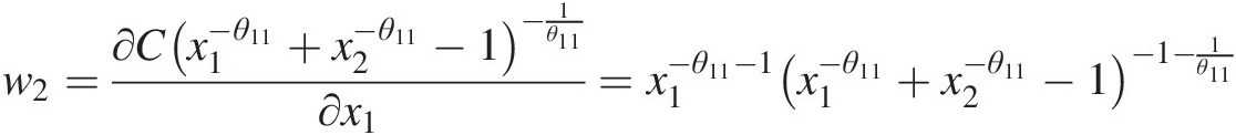
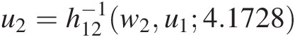
⇒x2=h−1w2x1θ11=1+x1−θ11w2−θ111+θ11−x1−θ11−1θ11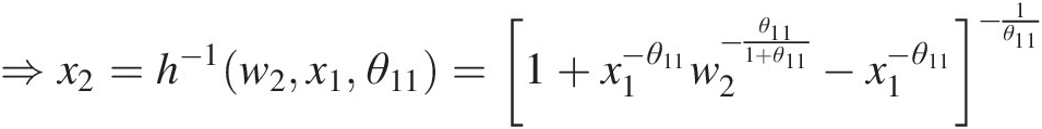
Substituting x1 = 0.1858, w2 = 0.1930, θ11 = 2.0x1=0.1858,w2=0.1930,θ11=2.0 into the preceding equation, we have the following:
x2 = 0.1304x2=0.1304.
c. Set w3 = F(x3| x1, x2) = h{h(x3, x1; θ12), h(x2, x1; θ11); θ21}w3=Fx3x1x2=hhx3x1θ12hx2x1θ11θ21, where
hx3x1θ12=t2=x1−θ12−1×1−θ12+x3−θ12−1−1−1θ12;
hx2x1θ11=t1=x1−θ11−1×1−θ11+x2−θ11−1−1−1θ11;
hhx3x1θ12hx2x1θ11θ21=t1−θ21−1t1−θ21+t2−θ21−1−1−1θ21
Substitute x1 = 0.1858, x2 = 0.1304, w3 = 0.3416, θ11 = 2.0, θ12 = 5.0, θ21 = 2.0x1=0.1858,x2=0.1304,w3=0.3416,θ11=2.0,θ12=5.0,θ21=2.0 to solve the nonlinear equation
x3 = h−1{h−1(0.3416, h(0.1304, 0.1858; 2.0); 2.0), 0.1858; 5.0}x3=h−1h−10.3416h0.13040.18582.02.00.18585.0, and we have the following:
x3 = 0.1484x3=0.1484.
Finally, we get the following:
(x1, x2, x3) = (0.1858, 0.1304, 0.1484)x1x2x3=0.18580.13040.1484.


5.3.5 Parameter Estimation for a Specified Pair-Copula Decomposition
Parameter estimation for specified pair-copula decomposition can be obtained using the log-likelihood method for the C-vine copula using the density function given by Equation (5.28) or D-vine copula with the density function given by Equation (5.27).
Parameter Estimation for a C-Vine Copula
From Equation (5.28), the log-likelihood expression of the C-vine copula is given as
 (5.39)
The log-likelihood in Equation (5.39) must be numerically maximized over all parameters using the algorithm 3 (Aas et al., 2009). As discussed earlier, for the d-dimensional Vine copula, we have T = {Ti : i = 1, …d − 1}T=Ti:i=1…d−1 levels. Within each level TiTi, we have EdgeTi = {Ej : j = 1, …, d − i}.EdgeTi=Ej:j=1…d−i. In other words, we have d − id−i bivariate unconditional/conditional copulas for each level TiTi. There are two loops in algorithm 3. The outer loop identifies the tree level, while the inner loop identifies the edges (i.e., the bivariate copulas) of each level. Using variable 1 as the center variable, the algorithm can be explained as follows:
Setting
x0 = [x1, …, xd] = [u1, …, ud], θ = [θ11, θ12, …θ(d − 1)1]x0=x1…xd=u1…ud,θ=θ11θ12…θd−11 and LL=0
Outer Loop: i = 1 to d − 1 (for level T)
Inner Loop: j = 1 to d − i (edges for each level)
c = copulapdf(xi − 1, 1, xi − 1, j + 1, θij);
LL = LL + ∑ ln (c);
xij = h(xi − 1, j + 1, xi − 1, 1; θij)
End Inner Loop
End Outer Loop
Parameter Estimation for a D-Vine Copula
For the D-vine copula, the log-likelihood function is given by
 (5.40)
Let Θj, iΘj,i be the set of parameters of the copula density Ci, i + j ∣ i + 1, …, i + j − 1(⋅, ⋅)Ci,i+j∣i+1,…,i+j−1⋅⋅. Algorithm 4 (Aas et al., 2009) evaluates the likelihood, which can be explained as follows:
Compute the log-likelihood (LL) for T1 and start the computation of conditional copulas:
Prepare the conditional probability for a higher level:
Update the log-likelihood as well as the conditional probability for a higher level:
stop the loop if i = d − 1i=d−1; otherwise, we will continue the loop
again stop the loop if d ≤ 4d≤4; otherwise we will continue on
To apply algorithms 3 and 4 to optimize the parameters, the initial values of the parameters are needed, which may be determined as follows (Aas et al., 2009):
a. Estimate parameters of the copulas in T1 from the original data.
b. Compute observations (i.e., conditional distribution functions) for T2 using the copula parameters from T1 and the corresponding h-function.
c. Estimate parameters of the copulas in T2 using the results computed from step b.
d. Compute observations for T3 using the copula parameters at T2 and the corresponding h-function.
e. Estimate the parameters of copulas in T3 using the results computed from step d.
…
f. Repeat the previous steps sequentially until we teach the top level of the vine tree, i.e., Td–1.
Parameter Estimation for Basic Three-Variable Model
For a three-dimensional special case (i.e., Figure 5.10(a)), the log-likelihood in Equation (5.39) and Equation (5.40) can be simply written as
 (5.41)
where v1, i = F(x1, i| x2, i) = h(x1, i, x2, i; Θ11)v1,i=Fx1,ix2,i=hx1,ix2,iΘ11 and v2, i = F(x3, i| x2, i) = h(x3, i, x2, i; Θ12)v2,i=Fx3,ix2,i=hx3,ix2,iΘ12; ΘjiΘji are the set of parameters of the corresponding copula density cj, j + i ∣ 1, …, j − 1(⋅| ⋅)cj,j+i∣1,…,j−1⋅⋅. Here we give some common h-functions.
For the Gumbel–Hougaard copula, the h-function can be given as
 (5.42)
where Cu1u2θ=e−−lnu1θ+−lnu2θ1θ . For the Clayton copula, the h-function can be expressed as
 (5.43)
For the Frank copula, the h-function can be written as
 (5.44)
For the Ali–Mikhail–Haq copula, the h-function can be cast as
 (5.45)
For the Gaussian copula, the h-function can be written as
 (5.46)
In Equation (5.46), ρ12ρ12 is the parameter of copula, i.e., the correlation coefficient for the bivariate random variables after meta-Gaussian transformation, and Φ−1()Φ−1 is the inverse of the standard univariate Gaussian distribution function.
For the Student t copula, the h-function can be given as
 (5.47)
In Equation (5.47), ρ12ρ12 and ν12ν12 are the parameters of Student t copula, i.e., the correlation coefficient and degree of freedom for the transformed variables using Student distribution with degree of freedom (d.f.) of ν12ν12; and Tν12−1⋅ is the inverse of Student T distribution with d.f. of ν12ν12, expectation 0, and variance ν12ν12−2
 .
.
Example 5.15 Assuming that the trivariate random variable given in Table 5.4 may be modeled by the Clayton–Clayton–Frank vine copula with the vine scheme shown in Figure 5.10(a), (1) estimate the parameters using the sequential MLE; and (2) simulate 50 samples from the fitted vine-copula function.
Table 5.4. Data and results for Example 5.14.
| u1u1 | u2u2 | u3u3 | h(u1, u2; θ11)hu1u2θ11 | h(u3, u2; θ12)hu3u2θ12 |
|---|---|---|---|---|
| 0.241 | 0.138 | 0.103 | 0.892 | 0.061 |
| 0.241 | 0.172 | 0.172 | 0.762 | 0.460 |
| 0.241 | 0.241 | 0.276 | 0.424 | 0.729 |
| 0.241 | 0.586 | 0.655 | 0.010 | 0.696 |
| 0.793 | 0.828 | 0.897 | 0.503 | 0.741 |
| 0.483 | 0.345 | 0.379 | 0.771 | 0.660 |
| 0.931 | 0.914 | 0.621 | 0.767 | 0.026 |
| 0.724 | 0.759 | 0.724 | 0.452 | 0.379 |
| 0.414 | 0.621 | 0.586 | 0.102 | 0.344 |
| 0.759 | 0.414 | 0.310 | 0.936 | 0.061 |
| 0.862 | 0.793 | 0.793 | 0.705 | 0.500 |
| 0.655 | 0.517 | 0.448 | 0.716 | 0.195 |
| 0.414 | 0.379 | 0.552 | 0.526 | 0.954 |
| 0.569 | 0.448 | 0.414 | 0.699 | 0.297 |
| 0.569 | 0.690 | 0.690 | 0.254 | 0.472 |
| 0.414 | 0.310 | 0.241 | 0.727 | 0.083 |
| 0.241 | 0.552 | 0.862 | 0.013 | 0.981 |
| 0.069 | 0.035 | 0.035 | 0.935 | 0.460 |
| 0.241 | 0.276 | 0.345 | 0.287 | 0.852 |
| 0.069 | 0.069 | 0.069 | 0.424 | 0.460 |
| 0.897 | 0.914 | 0.931 | 0.661 | 0.694 |
| 0.655 | 0.655 | 0.483 | 0.473 | 0.053 |
| 0.069 | 0.103 | 0.138 | 0.100 | 0.908 |
| 0.241 | 0.207 | 0.207 | 0.593 | 0.460 |
| 0.655 | 0.724 | 0.759 | 0.364 | 0.587 |
| 0.517 | 0.483 | 0.517 | 0.517 | 0.609 |
| 0.828 | 0.862 | 0.828 | 0.539 | 0.431 |
| 0.966 | 0.966 | 0.966 | 0.854 | 0.776 |
Solution:
1. Estimate the parameters. For the bivariate Clayton copula C(u, v; θ)Cuvθ, its copula density function can be given as follows:
cuvθ=1+θuθ+1vθ+1u−θ+v−θ−12+1θFor the bivariate Frank copula, its copula density function can be given as follows: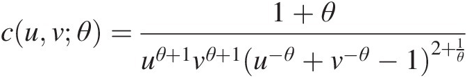 (5.48)
cuvθ=θe−θu+ve−θu−1e−θv−1e−θ−12s12−θe−θu+ve−θ−1s1;s1=e−θu−1e−θv−1e−θ−1+1 (5.49)
a. Estimate the parameters for T1.Using the maximum likelihood estimation for the Clayton copula, the copula parameters estimated for T1 can be estimated as follows:θ11 = 4.1728; θ12 = 8.3834θ11=4.1728;θ12=8.3834 for (u1, u2)u1u2 and (u2, u3)u2u3, respectively.
b. Compute the conditional distribution functions for T2 using the copula parameters estimated from T1. Using the h-function for the Clayton copula (Equation (5.43)) and parameters estimated for T1, we have the following:
hu1u2θ11=u2−5.1728u1−4.1728+u2−4.1728−1−1−14.1728
hu3u2θ12=u2−9.3834u2−8.3834+u3−8.3834−1−1−18.3834Table 5.4 lists the original datasets with the fourth and fifth columns as the computed conditional probabilities.
c. Estimate the parameter for T2 using the computed conditional probabilities from step b.


Similar to step a, using the maximum likelihood estimation for the Frank copula, the parameter estimated for T2 is estimated as θ21 = − 3.8431θ21=−3.8431.
2. Simulate 50 samples from the fitted vine-copula function:
Based on the algorithm 2 for sampling from the D-vine copula, we can simulate the samples from the fitted vine-copula as follows:
a. Generate independently uniform random variables {w1, w2, w3}.w1w2w3.
b. Set u1 = w1.u1=w1.
c. Use w2 = C(u2| u1) = h12(u2, u1; 4.1728)w2=Cu2u1=h12u2u14.1728 to compute u2=h12−1w2u14.1728
 using the h-function of the Clayton copula (Equation (5.43)).
d. Compute u3u3 with the following procedure:
Cu3u1u2=∂C13∣2C1∣2u1u2C3∣2u3u2θ21∂C1∣2u1u2=h13∣2h23u3u28.3834h12u1u24.1728−3.8431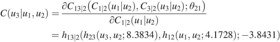
u3=h23−1h13∣2−1w3h12u1u24.1728− 3.8431u28.3834where h12, h23h12,h23 are h-functions for the Clayton copula at T1; h13 ∣ 2h13∣2 is the h-function for the Frank copula (Equation (5.44)) at T2.


Using the simulated samples and pseudo-observations, Figure 5.13 evaluated the performance of the fitted vine copula. it is seen that the pair-wise dependence is well preserved

Example 5.16 Using the four-dimensional pseudo-observations in Example 5.12 to (1) estimate the copula parameters using sequential MLE if D-vine copula (Figure 5.11(a)) with the specified copula (i.e., the Gumbel– Hougaard copula for T1 and the Frank copula for T2 and T3) and C-vine copula (Figure 5.11(b)) with specified copula (i.e., the Gumbel– Hougaard copula for T1, T2, and T3); and (2) simulate the random variates for the sample size of 100 from the fitted copulas.
Solution:
I. D-Vine Copula
1. Estimate the copula parameters:
The density function of the biviariate Gumbel–Hougaard and Frank copulas are given in Chapter 4 as follows:
Gumbel–Hougaard copula:
cuvθ=lnulnvθ−1e−S11θS12θ−2−1−θS11θ−2uv;S1=−lnuθ+−lnvθ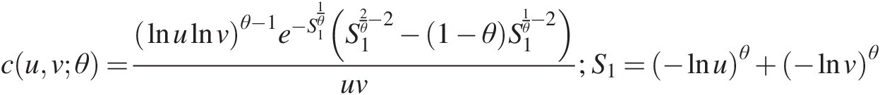 (5.50)
Frank copula: The same as the previous example, its copula density is given as Equation (5.49).
a. Estimate the parameters for the D-vine copula.
Estimation of copula parameters (the Gumbel–Hougaard copula) for T1:
For T1, applying the MLE, we have: θ11 = 3.8545, L11 = 59.783θ11=3.8545,L11=59.783 for (u1, u2)u1u2; θ12 = 3.0942, L12 = 49.653θ12=3.0942,L12=49.653 for (u2, u3)u2u3; θ13 = 4.3949, L13 = 71.727θ13=4.3949,L13=71.727 for (u3, u4)u3u4.
Estimation of copula parameters (Frank copula) for T2:
i. Compute the conditional distribution C1 ∣ 2(u1| U2 = u2; θ11 = 3.8545)C1∣2u1U2=u2θ11=3.8545, C3 ∣ 2(u3| U2 = u2; θ12 = 3.0942); C2 ∣ 3(u2| U3 = u3; θ12 = 3.0942);C3∣2u3U2=u2θ12=3.0942;C2∣3u2U3=u3θ12=3.0942; andC4 ∣ 3(u4| U3 = u3; θ13 = 4.3949)C4∣3u4U3=u3θ13=4.3949.
ii. Apply the MLE to estimate the parameters for T2 as follows: θ21 = 1.9708, L21 = 3.032θ21=1.9708,L21=3.032 for (C1 ∣ 2, C3 ∣ 2)C1∣2C3∣2; θ22 = 0.7916, L22 = 0.565θ22=0.7916,L22=0.565 for (C2 ∣ 3, C4 ∣ 3)C2∣3C4∣3.
Estimation of copula parameters (the Frank copula) for T3:
According to Figure 5.11(a), the copula function for T3 is given as follows: C14 ∣ 23(F(u1| u2, u3), F(u4| u2, u3))C14∣23Fu1u2u3Fu4u2u3
From Equation (5.24), we have the following:
Fu1u2u3=∂C13∣2Fu1u2Fu3u2∂Fu3u2;Fu4u2u3=∂C24∣3Fu2u3Fu4u3∂Fu2u3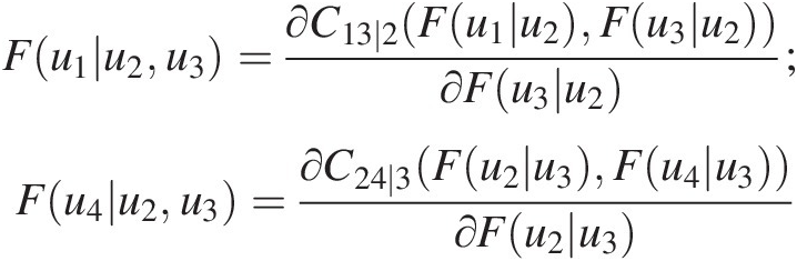


Using the parameters estimated for T1 and T2, we can easily calculate the conditional probability distribution needed for parameter estimation in T3. Maximizing the log-likelihood for the specified Frank copula, we have θ31 = − 0.4281, L31 = 0.173θ31=−0.4281,L31=0.173.
Finally, we have the following:
T1: θ11 = 3.8545; θ12 = 3.0942; θ13 = 4.3949θ11=3.8545;θ12=3.0942;θ13=4.3949
T2: θ21 = 1.9708; θ22 = 0.7916θ21=1.9708;θ22=0.7916
T3: θ31 = − 0.4281θ31=−0.4281
The overall log-likelihood is computed as the sum of all LL s: L = 184.933L=184.933. Table 5.5 lists the conditional probability distributions computed for T2 and T3 using the fitted copula of the previous level.
| T2 | T3 | ||||
|---|---|---|---|---|---|
| Cu2 ∣ u1Cu2∣u1 | Cu2 ∣ u3Cu2∣u3 | Cu3 ∣ u2Cu3∣u2 | Cu4 ∣ u3Cu4∣u3 | Cu1 ∣ u2,u3Cu1∣u2,u3 | Cu4 ∣ u2, u3Cu4∣u2,u3 |
| 0.143 | 0.327 | 0.654 | 0.830 | 0.099 | 0.851 |
| 0.134 | 0.971 | 0.089 | 0.387 | 0.237 | 0.302 |
| 0.470 | 0.613 | 0.499 | 0.703 | 0.469 | 0.687 |
| 0.524 | 0.258 | 0.638 | 0.456 | 0.458 | 0.504 |
| 0.722 | 0.200 | 0.910 | 0.799 | 0.554 | 0.837 |
| 0.307 | 0.445 | 0.625 | 0.291 | 0.246 | 0.298 |
| 0.220 | 0.665 | 0.149 | 0.346 | 0.340 | 0.316 |
| 0.500 | 0.106 | 0.949 | 0.118 | 0.292 | 0.152 |
| 0.102 | 0.487 | 0.409 | 0.119 | 0.107 | 0.118 |
| 0.736 | 0.122 | 0.749 | 0.929 | 0.648 | 0.948 |
| 0.742 | 0.486 | 0.487 | 0.701 | 0.761 | 0.705 |
| 0.654 | 0.588 | 0.414 | 0.821 | 0.702 | 0.814 |
| 0.773 | 0.651 | 0.058 | 0.575 | 0.899 | 0.546 |
| 0.143 | 0.535 | 0.307 | 0.780 | 0.179 | 0.777 |
| 0.760 | 0.196 | 0.888 | 0.220 | 0.615 | 0.261 |
| 0.601 | 0.529 | 0.713 | 0.712 | 0.505 | 0.710 |
| 0.177 | 0.040 | 0.991 | 0.725 | 0.068 | 0.794 |
| 0.593 | 0.209 | 0.674 | 0.084 | 0.516 | 0.101 |
| 0.401 | 0.697 | 0.497 | 0.965 | 0.395 | 0.960 |
| 0.507 | 0.843 | 0.092 | 0.756 | 0.698 | 0.706 |
| 0.690 | 0.376 | 0.749 | 0.125 | 0.592 | 0.134 |
| 0.254 | 0.802 | 0.313 | 0.945 | 0.313 | 0.933 |
| 0.143 | 0.386 | 0.193 | 0.943 | 0.214 | 0.949 |
| 0.467 | 0.191 | 0.796 | 0.296 | 0.326 | 0.347 |
| 0.265 | 0.376 | 0.821 | 0.482 | 0.151 | 0.506 |
| 0.908 | 0.361 | 0.693 | 0.806 | 0.884 | 0.825 |
| 0.809 | 0.261 | 0.575 | 0.096 | 0.801 | 0.112 |
| 0.891 | 0.052 | 0.969 | 0.761 | 0.786 | 0.821 |
| 0.345 | 0.880 | 0.081 | 0.305 | 0.534 | 0.243 |
| 0.015 | 0.934 | 0.055 | 0.817 | 0.031 | 0.763 |
| 0.145 | 0.754 | 0.020 | 0.833 | 0.281 | 0.806 |
| 0.762 | 0.985 | 0.071 | 0.683 | 0.890 | 0.597 |
| 0.989 | 0.140 | 0.771 | 0.440 | 0.984 | 0.510 |
| 0.164 | 0.801 | 0.319 | 0.443 | 0.202 | 0.384 |
| 0.026 | 0.887 | 0.144 | 0.902 | 0.045 | 0.873 |
| 0.032 | 0.991 | 0.048 | 0.792 | 0.065 | 0.724 |
| 0.101 | 0.693 | 0.409 | 0.985 | 0.106 | 0.983 |
| 0.713 | 0.159 | 0.722 | 0.948 | 0.632 | 0.961 |
| 0.163 | 0.137 | 0.659 | 0.042 | 0.113 | 0.054 |
| 0.309 | 0.231 | 0.609 | 0.286 | 0.254 | 0.329 |
| 0.177 | 0.784 | 0.293 | 0.579 | 0.226 | 0.524 |
| 0.731 | 0.301 | 0.812 | 0.113 | 0.613 | 0.128 |
| 0.099 | 0.071 | 0.968 | 0.508 | 0.037 | 0.592 |
| 0.072 | 0.211 | 0.399 | 0.209 | 0.077 | 0.246 |
| 0.320 | 0.413 | 0.737 | 0.126 | 0.218 | 0.132 |
| 0.190 | 0.015 | 0.991 | 0.874 | 0.075 | 0.912 |
| 0.047 | 0.873 | 0.224 | 0.245 | 0.069 | 0.193 |
| 0.363 | 0.899 | 0.250 | 0.086 | 0.472 | 0.063 |
| 0.566 | 0.375 | 0.664 | 0.843 | 0.492 | 0.857 |
| 0.383 | 0.614 | 0.602 | 0.692 | 0.328 | 0.675 |
| 0.041 | 0.525 | 0.625 | 0.095 | 0.028 | 0.091 |
| 0.863 | 0.437 | 0.750 | 0.267 | 0.813 | 0.274 |
| 0.096 | 0.225 | 0.862 | 0.805 | 0.044 | 0.840 |
| 0.461 | 0.424 | 0.290 | 0.108 | 0.560 | 0.112 |
| 0.805 | 0.595 | 0.297 | 0.149 | 0.871 | 0.137 |
| 0.555 | 0.470 | 0.505 | 0.058 | 0.557 | 0.058 |
| 0.414 | 0.312 | 0.873 | 0.486 | 0.248 | 0.523 |
| 0.191 | 0.929 | 0.210 | 0.510 | 0.274 | 0.425 |
| 0.449 | 0.783 | 0.124 | 0.602 | 0.628 | 0.549 |
| 0.785 | 0.327 | 0.852 | 0.403 | 0.666 | 0.435 |
Note: Cu1 ∣ u2, u3 = ∂C13 ∣ 2(Cu1 ∣ u2, Cu3 ∣ u2)/∂Cu3 ∣ u2Cu1∣u2,u3=∂C13∣2Cu1∣u2Cu3∣u2/∂Cu3∣u2; Cu4 ∣ u2, u3 = ∂C24 ∣ 3(Cu4 ∣ u3, Cu2 ∣ u3)/∂Cu2 ∣ u3Cu4∣u2,u3=∂C24∣3Cu4∣u3Cu2∣u3/∂Cu2∣u3.
II: C-Vine Copula
a. Estimation of copula parameters (the Gumbel–Hougaard copula) for T1:
According to Figure 5.11(b), we have the parameters estimated for T1 as follows: θ11 = 3.8545, L11 = 59.783θ11=3.8545,L11=59.783 for (u1, u2)u1u2; θ12 = 3.0834, L12 = 47.245θ12=3.0834,L12=47.245 for (u1, u3)u1u3; θ13 = 2.5704, L13 = 38.08θ13=2.5704,L13=38.08 for (u1, u4)u1u4.
b. Estimation of copula parameters (the Gumbel–Hougaard copula) for T2:
From Figure 5.11(b), we need to compute the conditional distribution using the parameter estimated from T1 first, and then we will be able to estimate the copula parameters for T2 as follows:
i. Compute the conditional distribution C2 ∣ 1(u2 ∣ U1 = u1; θ11 = 3.8545C2∣1(u2∣U1=u1;θ11=3.8545), C3 ∣ 1(u3| U1 = u1; θ12 = 3.0834)C3∣1u3U1=u1θ12=3.0834 and C4 ∣ 1(u4| U1 = u1; θ13 = 2.5704)C4∣1u4U1=u1θ13=2.5704.
ii. Apply the MLE to estimate the parameters for T2 as follows:
θ21 = 1.2618, L21 = 4.265θ21=1.2618,L21=4.265 for (C2 ∣ 1, C3 ∣ 1)C2∣1C3∣1;θ22 = 1.267, L22 = 4.356θ22=1.267,L22=4.356 for (C2 ∣ 1, C4 ∣ 1)C2∣1C4∣1.
c. Estimation of copula parameters (the Gumbel–Hougaard copula) for T3:
According to Figure 5.11(b), the copula function for T3 is given as C34 ∣ 12(F(u3| u1, u2), F(u4| u1, u2))C34∣12Fu3u1u2Fu4u1u2.
From Equation (5.24), we have the following:
Fu3u1u2=∂C23∣1Fu3u1Fu2u1∂Fu2u1;Fu4u1u2=∂C24∣1Fu4u1Fu2u1∂Fu2u1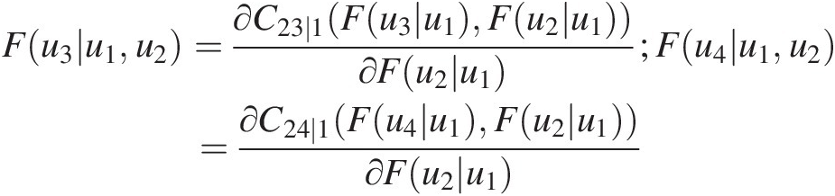
Using the parameters estimated for T1 and T2, we will first compute the conditional probability needed for parameter estimation in T3. Maximizing the log-likelihood for the specified Frank copula, we have θ31 = 1.959, L31 = 27.687θ31=1.959,L31=27.687.
Finally, we have the following:
T1: θ11 = 3.8545; θ12 = 3.0834; θ13 = 2.5704θ11=3.8545;θ12=3.0834;θ13=2.5704
T2: θ21 = 1.2618; θ22 = 1.2672θ21=1.2618;θ22=1.2672
T3: θ31 = 1.959θ31=1.959
The overall log-likelihood is computed as L = 181.416L=181.416. Table 5.6 lists the conditional probability distributions computed for T2 and T3.

Table 5.6. Conditional probability distributions computed for T2 and T3 of a fitted C-Vine copula.
| T2 | T3 | |||
|---|---|---|---|---|
| Cu2 ∣ u1Cu2∣u1 | Cu3 ∣ u1Cu3∣u1 | Cu4 ∣ u1Cu4∣u1 | Cu3 ∣ u1, u2Cu3∣u1,u2 | Cu4 ∣ u1, u2Cu4∣u1,u2 |
| 0.804 | 0.853 | 0.910 | 0.805 | 0.887 |
| 0.939 | 0.323 | 0.303 | 0.157 | 0.143 |
| 0.620 | 0.556 | 0.663 | 0.539 | 0.658 |
| 0.368 | 0.585 | 0.536 | 0.654 | 0.603 |
| 0.406 | 0.855 | 0.905 | 0.905 | 0.946 |
| 0.722 | 0.762 | 0.591 | 0.731 | 0.530 |
| 0.637 | 0.258 | 0.225 | 0.224 | 0.191 |
| 0.574 | 0.954 | 0.762 | 0.972 | 0.784 |
| 0.819 | 0.712 | 0.370 | 0.609 | 0.260 |
| 0.145 | 0.535 | 0.841 | 0.667 | 0.922 |
| 0.263 | 0.307 | 0.464 | 0.378 | 0.557 |
| 0.372 | 0.316 | 0.572 | 0.357 | 0.640 |
| 0.101 | 0.014 | 0.056 | 0.025 | 0.094 |
| 0.744 | 0.548 | 0.717 | 0.472 | 0.664 |
| 0.322 | 0.790 | 0.573 | 0.862 | 0.656 |
| 0.594 | 0.710 | 0.781 | 0.721 | 0.800 |
| 0.894 | 0.998 | 0.997 | 0.998 | 0.996 |
| 0.287 | 0.569 | 0.213 | 0.660 | 0.260 |
| 0.743 | 0.634 | 0.913 | 0.568 | 0.911 |
| 0.477 | 0.089 | 0.259 | 0.086 | 0.264 |
| 0.412 | 0.656 | 0.346 | 0.716 | 0.379 |
| 0.830 | 0.550 | 0.859 | 0.420 | 0.797 |
| 0.530 | 0.319 | 0.789 | 0.314 | 0.825 |
| 0.477 | 0.797 | 0.631 | 0.843 | 0.672 |
| 0.863 | 0.938 | 0.898 | 0.904 | 0.834 |
| 0.127 | 0.321 | 0.551 | 0.441 | 0.691 |
| 0.122 | 0.286 | 0.098 | 0.400 | 0.152 |
| 0.129 | 0.869 | 0.900 | 0.940 | 0.959 |
| 0.655 | 0.125 | 0.109 | 0.099 | 0.085 |
| 0.979 | 0.520 | 0.727 | 0.213 | 0.352 |
| 0.594 | 0.050 | 0.330 | 0.040 | 0.307 |
| 0.413 | 0.046 | 0.115 | 0.048 | 0.121 |
| 0.008 | 0.108 | 0.137 | 0.232 | 0.283 |
| 0.898 | 0.661 | 0.596 | 0.471 | 0.402 |
| 0.977 | 0.709 | 0.882 | 0.355 | 0.558 |
| 0.992 | 0.455 | 0.646 | 0.138 | 0.224 |
| 0.925 | 0.801 | 0.973 | 0.599 | 0.936 |
| 0.180 | 0.529 | 0.863 | 0.650 | 0.933 |
| 0.567 | 0.775 | 0.293 | 0.801 | 0.276 |
| 0.503 | 0.671 | 0.495 | 0.707 | 0.516 |
| 0.867 | 0.594 | 0.617 | 0.435 | 0.456 |
| 0.365 | 0.702 | 0.367 | 0.773 | 0.417 |
| 0.906 | 0.994 | 0.983 | 0.991 | 0.970 |
| 0.622 | 0.625 | 0.406 | 0.615 | 0.376 |
| 0.774 | 0.859 | 0.563 | 0.830 | 0.470 |
| 0.736 | 0.996 | 0.996 | 0.998 | 0.998 |
| 0.975 | 0.778 | 0.576 | 0.429 | 0.256 |
| 0.793 | 0.397 | 0.173 | 0.297 | 0.112 |
| 0.459 | 0.627 | 0.801 | 0.672 | 0.851 |
| 0.766 | 0.745 | 0.794 | 0.686 | 0.748 |
| 0.973 | 0.958 | 0.743 | 0.779 | 0.393 |
| 0.251 | 0.488 | 0.360 | 0.586 | 0.444 |
| 0.918 | 0.973 | 0.976 | 0.942 | 0.950 |
| 0.335 | 0.252 | 0.090 | 0.293 | 0.104 |
| 0.178 | 0.125 | 0.062 | 0.175 | 0.089 |
| 0.434 | 0.461 | 0.130 | 0.500 | 0.134 |
| 0.762 | 0.928 | 0.888 | 0.925 | 0.873 |
| 0.918 | 0.518 | 0.527 | 0.313 | 0.317 |
| 0.503 | 0.133 | 0.235 | 0.128 | 0.233 |
| 0.370 | 0.731 | 0.645 | 0.800 | 0.717 |
According to algorithm 2, we can simulate the random variates from the fitted D-vine copula as follows:
Step 1: Generate independent uniformly distributed random variables: {w1, w2, w3, w4}.w1w2w3w4.
Step 2: Simulate u1u1 by setting u1 = v11 = w1.u1=v11=w1.
Step 3: Simulate u2u2 by setting u2 = v21 = h−1(w2, u1; 3.8545),u2=v21=h−1w2u13.8545, where hh is the conditional probability distribution for the Gumbel–Hougaard copula.
Step 4: Simulate u3u3:
Calculate v22 = h(v11, v21; 3.8545) = h(u1, u2; 3.8545).v22=hv11v213.8545=hu1u23.8545.
Simulate u3u3 in the same way as in Example 5.14:
u3 = v31 = h−1(h−1(w3, v22; θ21), v21; θ12)u3=v31=h−1h−1w3v22θ21v21θ12
= h−1{h−1[w3, h(u1, u2; 3.8545); 1.9708], u2; 3.0942}=h−1h−1w3hu1u23.85451.9708u23.0942
Simulate u4u4 using the following procedure:
✓ Calculate v32v32, v33v33, and v34v34 using
v32 = h(v21, v31; θ12) = h(u2, u3; 3.0942)v32=hv21v31θ12=hu2u33.0942
v33 = h(v31, v21; θ12) = h(u3, u2; 3.0942)v33=hv31v21θ12=hu3u23.0942
v34 = h(v22, v33; θ21) = h{h(u1, u2; 3.8545), h(u3, u2; 3.0942); 1.9708}v34=hv22v33θ21=hhu1u23.8545hu3u23.09421.9708
✓ Finally simulate u4u4 using:
temp1 = h−1(w4, v34; θ31) = h−1(w4, v34; −0.4281)temp1=h−1w4v34θ31=h−1w4v34−0.4281
temp2 = h−1(temp1, v32; θ22) = h−1(temp1, v32; 0.7916)temp2=h−1temp1v32θ22=h−1temp1v320.7916
u4 = v41 = h−1(temp2, u3; θ13) = h−1(temp2, u3; 4.3949)u4=v41=h−1temp2u3θ13=h−1temp2u34.3949
Simulation from a fitted C-vine copula
To simulate random variates from the fitted C-vine copula, algorithm 1 is applied. By generating independent uniformly distributed random variables {w1, w2, w3, w4}w1w2w3w4, we can simulate u1 = v11u1=v11 and u2 = v21u2=v21 using the exact same procedure as that for simulation from the fitted D-vine copula. In what follows, we will discuss how to generate u3u3 and u4u4 using algorithm 1 in detail:
i. Simulateu3u3:
✓ Calculate v22v22, i.e., C2 ∣ 1C2∣1:
v22 = h(v21, v11; θ11) = h(u2, u1; 3.8545)v22=hv21v11θ11=hu2u13.8545
✓ Simulate u3u3 by computing temp = C3 ∣ 1temp=C3∣1 first:
From w3=C3∣1,2=∂C23∣1C3∣1C2∣1∂C2∣1=hC3∣1C2∣1θ21=hC3∣1v22θ21
 , we have the following:C3 ∣ 1 = temp = h−1(w3, v22; θ21) = h−1(w3, v22; 1.2618)C3∣1=temp=h−1w3v22θ21=h−1w3v221.2618, and
u3 = v31 = h−1(temp, v11; θ12) = h−1(temp, u1; 3.0834)u3=v31=h−1tempv11θ12=h−1tempu13.0834
ii. Similarly, we can simulate u4u4 as follows:
✓ Calculate v32v32 and v33v33:
v32 = h(v31, v11; θ12) = h(u3, u1; 3.0834)v32=hv31v11θ12=hu3u13.0834
v33 = h(v32, v22; θ21) = h(v32, v22; 1.2618)v33=hv32v22θ21=hv32v221.2618
✓ Simulate u4u4:
temp1 = h−1(w4, v33; θ31) = h−1(w4, v33; 1.9590)temp1=h−1w4v33θ31=h−1w4v331.9590
temp2 = h−1(temp1, v22; θ22) = h−1(temp1, v22; 1.2672)temp2=h−1temp1v22θ22=h−1temp1v221.2672
u4 = v41 = h−1(temp2, v11; θ13) = h−1(temp2, u1; 2.5704)u4=v41=h−1temp2v11θ13=h−1temp2u12.5704


Figure 5.14 (a) Comparison of pseudo-observations with those simulated from the fitted D-vine copula; (b) comparison of pseudo-observations with those simulated from the fitted C-vine copula.
Figure 5.14(b) compares the pseudo-observations with those simulated from the fitted C-vine copula.
For the simulation of random variates, the inverse of the hh function is evaluated numerically for both D-vine and C-vine copulas.
Based on the overall log-likelihood computed in this example, we see that the log-likelihood value for the D-vine copula is slightly higher than that for the C-vine copula. Simulation plots show similar results between the fitted D-vine and C-vine copulas.
5.3.6 Selection of Vine Copula Structure
Previously, we have discussed how to estimate the parameters for the specified vine copula structure. Following Aas et al. (2009), for the estimation of pair-copula decomposition, we should consider (i) the selection of pair-copula decompositions; (ii) the selection of pair-copula types; and (iii) the estimation of copula parameters. In principle, we may use all the possible decompositions to estimate the copula parameters and to choose the best-fitted vine copula structure for a given d-dimensional variable. However, in reality with higher dimensions (i.e., d ≥ 3)d≥3), the number of possible decompositions increases significantly as d ! /2d!/2 (i.e., 3 C-Vine (D-Vine) copulas for three-dimensional variables, 12 D-vine and 12 C-vine copulas for four-dimensional variables, 60 D-vine and 60 C-vine copulas for five-dimensional variables, etc.). To avoid the evaluations for all possible decompositions, we may first look at the rank-based correlation structure, starting from T1, to achieve the proper vine decomposition.
Similar to the discussion in Section 5.3.5, with the proper study of rank-based correlation structure, we can modify the model selection using sequential MLE (Aas et al., 2009) for decomposition with the tree levels {T1, T2, …, Td − 1}T1T2…Td−1 in what follows:
1. Select the copula family and estimate the parameters for T1T1 using the original data: (a) the parameters may be estimated using MLE; (b) the best-fitted copula can be selected by minimizing AIC or BIC and assessed with the goodness-of-fit study that will be discussed in Section 5.3.7.
2. Transform observations required in T2T2 with the use of the copula fitted in T1T1 and its corresponding h(⋅)h⋅ function.
3. Select the copula family and estimate the parameters for T2T2. The best-fitted copula in T2T2 is selected in the same way as in T1T1.
4. Repeat steps 2 and 3 until we reach Td − 1Td−1.
Based on the previously discussed model selection, we know the copulas selected do not need to belong to the same copula families (D-vine copula in Example 5.15, as an example). In addition, we should note that the sequential MLE may not result in a globally optimal solution. To avoid this problem, we may estimate all the parameters simultaneously using algorithm 3 for C-vine (algorithm 4 for D-vine) copulas for the selected vine structure with the parameters estimated using the sequential MLE as the initial estimates. Here, we will show how to estimate the parameters simultaneously.
Example 5.17 Re-work Example 5.16: (1) estimate the copula parameters simultaneously using the same decomposition and copula families as Example 5.16; and (2) simulate the random variates for the sample size of 100 from the fitted copula functions.
Solution:
Estimate the copula parameters simultaneously.
Estimate the parameters for D-vine copula.
In Example 5.16, we have estimated the copula parameters sequentially for the D-vine copula as follows:
T1 : θ11 = 3.8545; θ12 = 3.0942; θ13 = 4.3949T1:θ11=3.8545;θ12=3.0942;θ13=4.3949 (the Gumbel–Hougaard copula family)
T2 : θ21 = 1.9708; θ22 = 0.7916T2:θ21=1.9708;θ22=0.7916 (the Frank copula family)
T3 : θ31 = − 0.4281T3:θ31=−0.4281 (the Frank copula family)
L1=∑i=1nlnc12u1iu2iθ11+lnc23u2iu3iθ12+lnc34u3iu4iθ13
v11 = h(u1, u2; θ11); v12 = h(u3, u2; θ12); v13 = h(u2, u3; θ12); v14 = h(u4, u3; θ13)v11=hu1u2θ11;v12=hu3u2θ12;v13=hu2u3θ12;v14=hu4u3θ13
L2=∑i=1nlnc13∣2v11iv12iθ21+lnc34∣2v13iv14iθ22
v21 = h(v11, v12; θ21); v22 = h(v14, v13; θ22)v21=hv11v12θ21;v22=hv14v13θ22
L3=∑i=1nlnc14∣23v21iv22iθ31Finally, we have the overall log-likelihood as L = L1 + L2 + L3L=L1+L2+L3, where n is the sample size.
Using the parameters estimated sequentially as initial estimates, we obtain the parameters simultaneously by maximizing the final LL (or equivalently minimizing –L):
θ11 = 3.7723, θ12 = 3.1705, θ13 = 4.3913, θ21 = 1.9931, θ22 = 0.7811, θ31 = − 0.4325θ11=3.7723,θ12=3.1705,θ13=4.3913,θ21=1.9931,θ22=0.7811,θ31=−0.4325
Overall log-likelihood is L = L1 + L2 + L3 = 184.988L=L1+L2+L3=184.988
AIC = − 2L + 2length(Θ) = − 2(184.988) + 2(6) = − 357.976AIC=−2L+2lengthΘ=−2184.988+26=−357.976
BIC = − 2L + ln (n)length(Θ) = − 2(184.988) + ln (60)(6) = − 345.409BIC=−2L+lnnlengthΘ=−2184.988+ln606=−345.409
Estimate the parameters for C-vine copula.
In Example 5.16, we have estimated the copula parameters sequentially for the C-vine copula as follows:
T1 : θ11 = 3.8545; θ12 = 3.0834; θ13 = 2.5704T1:θ11=3.8545;θ12=3.0834;θ13=2.5704 (the Gumbel–Hougaard copula family)
T2 : θ21 = 1.2618; θ22 = 1.2672T2:θ21=1.2618;θ22=1.2672 (the Gumbel–Hougaard copula family)
T3 : θ31 = 1.9590T3:θ31=1.9590 (the Gumbel–Hougaard copula family)
L1=∑i=1nlnc12u1iu2iθ11+lnc13u1iu3iθ12+lnc14u1iu4iθ13
v11 = h(u2, u1; θ11); v12 = h(u3, u1, θ12); v13 = h(u4, u1; θ13)v11=hu2u1θ11;v12=hu3u1θ12;v13=hu4u1θ13
L2=∑i=1nlnc23∣1v11iv12iθ21+lnc24∣1v11v13θ22
v21 = h(v12, v11; θ21); v22 = h(v13, v11; θ22)v21=hv12v11θ21;v22=hv13v11θ22
Finally, we have the overall log-likelihood as L = L1 + L2 + L3L=L1+L2+L3.
L3 = ln (c34 ∣ 12(v21, v22; θ31))L3=lnc34∣12v21v22θ31
Again, using the parameters estimated sequentially as initial estimates from Example 5.16, we can estimate the parameters simultaneously by maximizing LL (or minimizing –L) as follows:
θ11 = 3.9280, θ12 = 2.9592, θ13 = 2.5509, θ21 = 1.2463, θ22 = 1.2285, θ31 = 2.0333θ11=3.9280,θ12=2.9592,θ13=2.5509,θ21=1.2463,θ22=1.2285,θ31=2.0333
The log-likelihood is evaluated as follows: L = 181.673, AIC = − 351.346, BIC = − 338.780L=181.673,AIC=−351.346,BIC=−338.780.
From the log-likelihood value, we see that the log-likelihood value obtained from the D-vine copula is slightly higher than that obtained from the C-vine copula. The AIC and BIC values (D-vine) are slightly smaller than those for the C-vine copula.
Simulate random variates
Using the same procedure as in Example 5.16, Figures 5.15(a) and 5.15(b), compare pseudo-observations with those simulated from the D-vine and C-vine copulas, respectively. The simulation plots show a similar comparison between the fitted D-vine and C-vine copulas.


Figure 5.15 (a) Comparison of pseudo-observations with those simulated from the fitted D-vine copula; (b) comparison of pseudo-observations with those simulated from the fitted C-vine copula.
Comparing with Example 5.16, there are minimal differences for the log-likelihood value, AIC and BIC obtained for D-vine and C-vine copulas. In addition, the sequential estimation method is more direct and easier to apply than is the simultaneous estimation method.
5.3.7 Goodness-of-Fit Test
Aas et al. (2009) proposed to use the probability integral transform (PIT, i.e., Rosenblatt’s transform) to test the goodness-of-fit for the pair-copula decomposition. Previously, in Section 5.2.5 we have discussed Rosenblatt’s transform. In what follows, we will illustrate the PIT algorithm for the C-vine and D-vine copulas (Aas et al., 2009). For a d-dimensional random variable x = {x1, x2, …xi…, , xn}, xi = {xi, 1, …, xi, d}x=x1x2…xi…xn,xi=xi,1…xi,d, the PIT is defined as follows:
 (5.51)
For a C-vine copula, the conditional distribution is computed using Equation (5.37) as given in algorithm 5 (Aas et al., 2009) that may be explained with dd-dimensional copula variable of sample size nn, as follows:
1. Set z1, 1 = x1, 1 = u1, 1z1,1=x1,1=u1,1. Here the first subscript represents the dimension, and second represents the sample considered.
2. Use loops to compute zi, i = 2, …, dzi,i=2,…,d.
for i = 2 to dfori=2tod
zi, 1 = xi, 1zi,1=xi,1
for j = 1 to d − 1forj=1tod−1
zi, 1 = h(temp, zj, 1; θj, i − j)zi,1=htempzj,1θj,i−j
endend
endend
3. Repeat steps 1 and 2 n times.
The D-vine copula applies Equation (5.38) to compute the conditional distributions for PIT, which is given as algorithm 6 in Aas et al. (2009). It again may be explained for a dd-dimensional D-vine copula variables of sample size nn using x1 = [x11, x21, …, xd1]x1=x11x21…xd1 as follows:
1. Set z11 = x11 = u11z11=x11=u11. The subscripts are defined exactly same as those in algorithm 5.
2. Compute the conditional distribution of z2, 1 = C2 ∣ 1z2,1=C2∣1 and C1 ∣ 2C1∣2:
z21 = h(x21, x11; θ11);z21=hx21x11θ11;
setting s21 = x21;settings21=x21;
computings22 = h(x11, x21; θ11)computing s22=hx11x21θ11
3. Compute the conditional distribution for x31|x11, x21, …xd1|x11,. . x(d − 1)1x31x11x21…xd1x11,..xd−11:
for i = 3 to dfori=3tod
zi1 = h(xi1, x(i − 1)1; θ1(i − 1))zi1=hxi1xi−11θ1i−1 % temporary: representing Ci ∣ i − 1Ci∣i−1.
for j = 2 to i − 1forj=2toi−1
zi1 = h(zi1, si − 1, 2(j − 1); θj, i − j)zi1=hzi1si−1,2j−1θj,i−j
endend
stop if i = di=d. Otherwise we need to continue the loop
set si1 = xi1; si2 = h(s(i − 1)1, si1; θ1(i − 1)); si3 = h(si1, s(i − 1)1; θ1(i − 1))si1=xi1;si2=hsi−11si1θ1i−1;si3=hsi1si−11θ1i−1
for j = 1 to i − 3forj=1toi−3
si(2j + 2) = h(s(i − 1)2j, si(2j + 1); θ(j + 1)(i − j − 1));si2j+2=hsi−12jsi2j+1θj+1i−j−1;
si(2j + 3) = h(si(2j + 1), s(i − 1)2j; θ(j + 1)(i − j − 1))si2j+3=hsi2j+1si−12jθj+1i−j−1
end
si(2i − 2) = h(s(i − 1)(2i − 4), si(2i − 3); θ(i − 1)1)si2i−2=hsi−12i−4si2i−3θi−11
end
4. Repeat steps 1–3 n times.
With the use of the PIT, the goodness-of-fit test may be performed in two ways: by applying the Anderson–Darling test and by applying the new procedure based on PIT proposed by Genest et al. (2007b).
Applying the Anderson–Darling Test
Compared to the new procedure proposed by Genest et al. (2007b), the Anderson–Darling test has inferior performance. However, we are still going to introduce this formal test here. Using the variables after PIT, we define the following:
 (5.52a)
where χ2χ2 follows the chi-square distribution with the degree of freedom (d.f.= d; i.e., the dimension of the multivariate random variable). The nonparametric CDF of χ2χ2 computed from Equation (5.52a) may then be estimated as follows:
 (5.52b)
Under the null hypothesis of Zs being independent and uniformly distributed, the Anderson–Darling test statistic is given as (Genest et al., 2007a):
 (5.53)
where χ12≤…≤χn2 are the order statistics corresponding to χ12,…χn2
 .
.
To avoid the misidentification of the limiting probability distribution, the P-value is estimated using the parametric bootstrap method for large integer N. Repeat the following steps for every k ∈ {1, …, N}k∈1…N:
a. Generate a random sample X1,k∗,…,Xn,k∗
 from the vine copula CθnCθn and compute their associated rank vectors: R1,k∗,…,Rn,k∗
 .
.
b. Compute Ui,k∗=Ri,k∗/n+1
 for i ∈ {1, …, n}i∈1…n.
c. Reestimate parameters (i.e., θn,k∗
 ) for the vine copula using U1,k∗…Un,k∗
 and compute χk∗={χ1,k2∗,…,χn,k2∗
 }, where χi,k2∗=∑j=1dΦ−1Zij,k∗2
 with Zij,k∗
 is determined from algorithm 5 or 6 (or simply using Equation (5.11)).
d. Compute the Anderson–Darling test statistics Ak∗
 using χk∗
 from Equation (5.53).


The approximate P-value for the test is then given by ∑k=1N1Ak∗>A/N .
.
Applying the New Procedure Based on PIT Proposed by Genest et al. (2007b)
As discussed in Section 4.7.1, the null hypothesis is ZZ (after Rosenblatt’s transform), being close to C⊥C⊥, where Z = {Z1, …Zi, …, Zn}, Zi = {Z1, Z2, …, Zd}Z=Z1…Zi…Zn,Zi=Z1Z2…Zd as follows:
1. Compute DnDn and test statistics SnB
 using the fitted copula model as follows:
Dnu=1n∑i=1nZi≤u,u∈01d (5.54)
SnB=n∫01dDnu−C⊥u2du=n3d−12d−1∑i=1n∏k=1d1−Zik2+1n∑i=1n∑j=1n∏k=1d1−Zik∨Zjk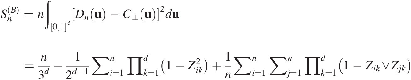 (5.55)
where Zik ∨ Zjk = max (Zik, Zjk)Zik∨Zjk=maxZikZjk.
2. For some large integer N, repeat the following steps for k = {1, 2, …, N}k=12…N:
a. Generate a random sample X1,k∗,…,Xn,k∗
 from the vine copula CθnCθn and compute their associated rank vectors: R1,k∗,…,Rn,k∗
 .
.
b. Compute Ui,k∗=Ri,k∗/n+1
 for i ∈ {1, …, n}.i∈1…n.
c. Reestimate parameters (i.e., θn,k∗
 ) for the vine copula using U1,k∗…Un,k∗
 and compute Z1,k∗,…,Zn,k∗
 using an appropriate algorithm (algorithm 5 or 6) or simply using Equation (5.11).
d. Compute Dn,k∗
 and Sn,kB∗
 using Equations (5.54) and (5.55) with reestimated parameter θn,k∗
 .
.


The appropriate P-value for the test is then given as follows: ∑k=1N1Sn,kB∗>SnB/N .
.
Example 5.18 Assess the GoF for the C- or D-vine copula constructed in Example 5.15 for trivariate analysis with both the Anderson–Darling test and the new procedure based on PIT proposed by Genest et al. (2007b) discussed in the preceding section.
Solution: Previously, we have shown that in the case of trivariate random variables, it is indifferent between C- and D-vine copulas. From Example 5.15, we have estimated the parameters for the Clayton–Clayton–Frank copula sequentially as follows:
T1: Clayton copula— θ11 = 4.1728 (u1, u2); θ12 = 8.3834 (u2, u3)θ11=4.1728u1u2;θ12=8.3834u2u3
T2: Frank copula— θ21 = − 3.8431 (C1 ∣ 2, C3 ∣ 2)θ21=−3.8431C1∣2C3∣2
Based on the Rosenblatt transform, Equation (5.53) may be rewritten for the three-dimensional C- or D-vine copulas as follows:
 (5.56)
With the estimated parameters using the sequential MLE and Equation (5.56), Table 5.7 lists Zs along with test statistics.
Table 5.7. Computed Zs and corresponding test statistics for three-dimensional C- or D-vine copulas.
| Observed | |||||
|---|---|---|---|---|---|
| u1 | u2 | u3 | Z1 | Z2 | Z3 |
| 0.241 | 0.138 | 0.103 | 0.241 | 0.049 | 0.152 |
| 0.241 | 0.172 | 0.172 | 0.241 | 0.134 | 0.690 |
| 0.241 | 0.241 | 0.276 | 0.241 | 0.424 | 0.723 |
| 0.241 | 0.586 | 0.655 | 0.241 | 0.973 | 0.304 |
| 0.793 | 0.828 | 0.897 | 0.793 | 0.627 | 0.793 |
| 0.483 | 0.345 | 0.379 | 0.483 | 0.135 | 0.869 |
| 0.931 | 0.914 | 0.621 | 0.931 | 0.696 | 0.042 |
| 0.724 | 0.759 | 0.724 | 0.724 | 0.575 | 0.306 |
| 0.414 | 0.621 | 0.586 | 0.414 | 0.833 | 0.087 |
| 0.759 | 0.414 | 0.310 | 0.759 | 0.041 | 0.176 |
| 0.862 | 0.793 | 0.793 | 0.862 | 0.458 | 0.687 |
| 0.655 | 0.517 | 0.448 | 0.655 | 0.211 | 0.281 |
| 0.414 | 0.379 | 0.552 | 0.414 | 0.336 | 0.974 |
| 0.569 | 0.448 | 0.414 | 0.569 | 0.204 | 0.419 |
| 0.569 | 0.690 | 0.690 | 0.569 | 0.687 | 0.252 |
| 0.414 | 0.310 | 0.241 | 0.414 | 0.164 | 0.120 |
| 0.241 | 0.552 | 0.862 | 0.241 | 0.965 | 0.933 |
| 0.069 | 0.034 | 0.034 | 0.069 | 0.026 | 0.813 |
| 0.241 | 0.276 | 0.345 | 0.241 | 0.572 | 0.790 |
| 0.069 | 0.069 | 0.069 | 0.069 | 0.423 | 0.378 |
| 0.897 | 0.914 | 0.931 | 0.897 | 0.730 | 0.841 |
| 0.655 | 0.655 | 0.483 | 0.655 | 0.473 | 0.029 |
| 0.069 | 0.103 | 0.138 | 0.069 | 0.811 | 0.771 |
| 0.241 | 0.207 | 0.207 | 0.241 | 0.267 | 0.538 |
| 0.655 | 0.724 | 0.759 | 0.655 | 0.611 | 0.482 |
| 0.517 | 0.483 | 0.517 | 0.517 | 0.362 | 0.653 |
| 0.828 | 0.862 | 0.828 | 0.828 | 0.665 | 0.448 |
| 0.966 | 0.966 | 0.966 | 0.966 | 0.854 | 0.949 |
Notes:
Anderson–Darling test statistic: An = 0.3572, P = 0.878 (with N = 1,000).
Rosenblatt (SnB) test statistic: SnB = 0.0417, P = 0.532 (with N = 1,000).
The formal GoF results using the Anderson–Darling and SnB tests show that with 1,000 parametric bootstrap simulations, the fitted Clayton–Clayton–Frank copula may properly model the dependence of the studied trivariate random variables.
Example 5.19 Assess the GoF for the D- and C-vine copulas constructed in Example 5.16 with both of the two GoF approaches previously discussed.
Solution:
For the four-dimensional random variable, the parameters were estimated sequentially for the D-vine copula in Example 5.16 as follows:
T1:T1: Gumbel–Hougaard copula
θ11 = 3.8545 (u1, u2), θ12 = 3.0942 (u2, u3), θ13 = 4.3949 (u3, u4);θ11=3.8545u1u2,θ12=3.0942u2u3,θ13=4.3949u3u4;
θ21 = 1.9708 (C1 ∣ 2, C3 ∣ 2), θ22 = 0.7916 (C2 ∣ 3, C4 ∣ 3);θ21=1.9708C1∣2C3∣2,θ22=0.7916C2∣3C4∣3;
T3:T3: Frank copula
θ31 = − 0.4281 (C1 ∣ 23, C4 ∣ 23)θ31=−0.4281C1∣23C4∣23.
Now based on the PIT, Equation (5.53) can be rewritten for the four-dimensional D-vine copula as follows:
Z1=u1Z2=Cu2U1=u1=∂Cu1u2θ11∂u1Z3=Cu3U1=u1U2=u2=∂C13∣2C3∣2C1∣2∂C1∣2Z4=Cu4U1=u1U2=u2U3=u3=∂C14∣23C4∣23C1∣23∂C1∣23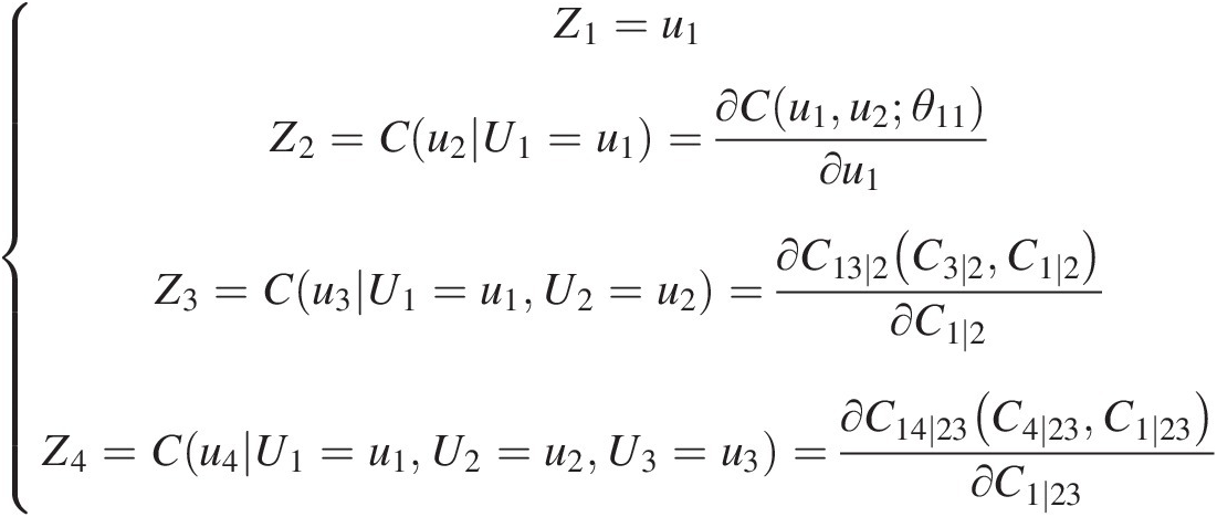 (5.57)
Table 5.8 lists the computed values from PIT using Equation (5.57) with the fitted four-dimensional D-vine copula.

Table 5.8. Computed Zs and corresponding test statistics for the D-vine copula.
| Z1Z1 | Z2Z2 | Z3Z3 | Z4Z4 |
|---|---|---|---|
| 0.194 | 0.804 | 0.801 | 0.828 |
| 0.819 | 0.939 | 0.150 | 0.278 |
| 0.614 | 0.620 | 0.513 | 0.685 |
| 0.235 | 0.368 | 0.638 | 0.499 |
| 0.792 | 0.406 | 0.882 | 0.841 |
| 0.433 | 0.722 | 0.717 | 0.275 |
| 0.130 | 0.638 | 0.214 | 0.301 |
| 0.570 | 0.574 | 0.956 | 0.141 |
| 0.128 | 0.819 | 0.596 | 0.101 |
| 0.218 | 0.145 | 0.670 | 0.951 |
| 0.468 | 0.263 | 0.370 | 0.729 |
| 0.490 | 0.373 | 0.337 | 0.827 |
| 0.194 | 0.102 | 0.030 | 0.588 |
| 0.120 | 0.744 | 0.458 | 0.754 |
| 0.676 | 0.322 | 0.843 | 0.271 |
| 0.990 | 0.589 | 0.683 | 0.713 |
| 0.657 | 0.894 | 0.996 | 0.762 |
| 0.226 | 0.287 | 0.646 | 0.101 |
| 0.828 | 0.743 | 0.546 | 0.959 |
| 0.373 | 0.477 | 0.081 | 0.724 |
| 0.698 | 0.412 | 0.690 | 0.138 |
| 0.645 | 0.830 | 0.410 | 0.928 |
| 0.025 | 0.531 | 0.304 | 0.943 |
| 0.298 | 0.477 | 0.820 | 0.330 |
| 0.906 | 0.863 | 0.890 | 0.470 |
| 0.658 | 0.127 | 0.519 | 0.848 |
| 0.302 | 0.122 | 0.430 | 0.125 |
| 0.581 | 0.129 | 0.943 | 0.839 |
| 0.371 | 0.655 | 0.095 | 0.245 |
| 0.169 | 0.980 | 0.115 | 0.726 |
| 0.041 | 0.594 | 0.034 | 0.791 |
| 0.982 | 0.410 | 0.039 | 0.637 |
| 0.585 | 0.008 | 0.584 | 0.562 |
| 0.618 | 0.898 | 0.462 | 0.354 |
| 0.280 | 0.977 | 0.276 | 0.851 |
| 0.902 | 0.992 | 0.098 | 0.686 |
| 0.440 | 0.925 | 0.596 | 0.981 |
| 0.243 | 0.180 | 0.647 | 0.963 |
| 0.044 | 0.567 | 0.798 | 0.046 |
| 0.122 | 0.503 | 0.701 | 0.306 |
| 0.497 | 0.867 | 0.423 | 0.495 |
| 0.701 | 0.365 | 0.752 | 0.133 |
| 0.323 | 0.906 | 0.987 | 0.544 |
| 0.013 | 0.622 | 0.599 | 0.214 |
| 0.651 | 0.774 | 0.812 | 0.118 |
| 0.190 | 0.736 | 0.996 | 0.897 |
| 0.520 | 0.975 | 0.393 | 0.165 |
| 0.926 | 0.793 | 0.287 | 0.062 |
| 0.468 | 0.459 | 0.646 | 0.858 |
| 0.868 | 0.766 | 0.663 | 0.660 |
| 0.422 | 0.973 | 0.811 | 0.076 |
| 0.888 | 0.251 | 0.613 | 0.301 |
| 0.372 | 0.918 | 0.940 | 0.812 |
| 0.132 | 0.335 | 0.293 | 0.114 |
| 0.429 | 0.178 | 0.179 | 0.156 |
| 0.390 | 0.434 | 0.478 | 0.059 |
| 0.983 | 0.765 | 0.902 | 0.495 |
| 0.980 | 0.917 | 0.310 | 0.401 |
| 0.308 | 0.503 | 0.122 | 0.562 |
| 0.932 | 0.370 | 0.786 | 0.452 |
Notes:
An (Equation 4.55): An = 0.7411, P-value = 0.261.
SnB (Equation 4.56): SnB = 0.0362, P-value = 0.08.
To approximate the P-value using the parametric bootstrap simulation method, we will use N = 1,000 as an example. It is known that the larger the N value, the closer to the true P-value for the GoF study.
For the four-dimensional random variable, parameters were estimated sequentially for the C-vine copula in Example 5.15 as follows:
T1 (Gumbel): θ11 = 3.8545, (u1, u2)θ11=3.8545,u1u2; θ12 = 3.0834, (u1, u3)θ12=3.0834,u1u3; θ13 = 2.5704, (u1, u4)θ13=2.5704,u1u4.
T2 (Gumbel): θ21 = 1.2618 (C2 ∣ 1, C3 ∣ 1); θ22 = 1.2672 (C2 ∣ 1, C4 ∣ 1)θ21=1.2618C2∣1C3∣1;θ22=1.2672C2∣1C4∣1
T3 (Gumbel): θ31 = 1.9590 (C3 ∣ 12, C4 ∣ 12)θ31=1.9590C3∣12C4∣12
According to the C-vine structure, the PIT of Equation (5.57) is rewritten as follows:
 (5.58)
Table 5.9 lists the computed Zs and corresponding test statistics for the fitted C-vine copula.
Table 5.9. Computed Zs and the corresponding test statistics for the fitted C-vine copula.
| Z1Z1 | Z2Z2 | Z3Z3 | Z4Z4 |
|---|---|---|---|
| 0.194 | 0.804 | 0.805 | 0.846 |
| 0.819 | 0.939 | 0.157 | 0.296 |
| 0.614 | 0.620 | 0.539 | 0.727 |
| 0.235 | 0.368 | 0.654 | 0.511 |
| 0.792 | 0.406 | 0.905 | 0.859 |
| 0.433 | 0.722 | 0.731 | 0.306 |
| 0.130 | 0.638 | 0.223 | 0.319 |
| 0.570 | 0.574 | 0.972 | 0.102 |
| 0.128 | 0.819 | 0.609 | 0.140 |
| 0.218 | 0.145 | 0.667 | 0.971 |
| 0.468 | 0.263 | 0.378 | 0.724 |
| 0.490 | 0.373 | 0.357 | 0.832 |
| 0.194 | 0.102 | 0.025 | 0.409 |
| 0.120 | 0.744 | 0.472 | 0.786 |
| 0.676 | 0.322 | 0.862 | 0.257 |
| 0.990 | 0.589 | 0.719 | 0.771 |
| 0.657 | 0.894 | 0.998 | 0.461 |
| 0.226 | 0.287 | 0.660 | 0.114 |
| 0.828 | 0.743 | 0.568 | 0.978 |
| 0.373 | 0.477 | 0.086 | 0.617 |
| 0.698 | 0.412 | 0.717 | 0.169 |
| 0.645 | 0.830 | 0.420 | 0.936 |
| 0.025 | 0.531 | 0.314 | 0.969 |
| 0.298 | 0.477 | 0.843 | 0.314 |
| 0.906 | 0.863 | 0.904 | 0.448 |
| 0.658 | 0.127 | 0.441 | 0.838 |
| 0.302 | 0.122 | 0.401 | 0.137 |
| 0.581 | 0.129 | 0.940 | 0.816 |
| 0.371 | 0.655 | 0.098 | 0.231 |
| 0.169 | 0.980 | 0.213 | 0.596 |
| 0.041 | 0.594 | 0.041 | 0.749 |
| 0.982 | 0.410 | 0.048 | 0.416 |
| 0.585 | 0.008 | 0.232 | 0.469 |
| 0.618 | 0.898 | 0.471 | 0.416 |
| 0.280 | 0.977 | 0.354 | 0.743 |
| 0.902 | 0.992 | 0.138 | 0.476 |
| 0.440 | 0.925 | 0.599 | 0.987 |
| 0.243 | 0.180 | 0.650 | 0.981 |
| 0.044 | 0.567 | 0.801 | 0.062 |
| 0.122 | 0.503 | 0.707 | 0.318 |
| 0.497 | 0.867 | 0.435 | 0.531 |
| 0.701 | 0.365 | 0.774 | 0.154 |
| 0.323 | 0.906 | 0.991 | 0.289 |
| 0.013 | 0.622 | 0.614 | 0.249 |
| 0.651 | 0.774 | 0.830 | 0.140 |
| 0.190 | 0.736 | 0.998 | 0.728 |
| 0.520 | 0.975 | 0.429 | 0.250 |
| 0.926 | 0.793 | 0.297 | 0.135 |
| 0.468 | 0.459 | 0.673 | 0.895 |
| 0.868 | 0.766 | 0.686 | 0.717 |
| 0.422 | 0.973 | 0.779 | 0.133 |
| 0.888 | 0.251 | 0.586 | 0.360 |
| 0.372 | 0.918 | 0.942 | 0.742 |
| 0.132 | 0.335 | 0.293 | 0.125 |
| 0.429 | 0.178 | 0.175 | 0.168 |
| 0.390 | 0.434 | 0.500 | 0.081 |
| 0.983 | 0.765 | 0.925 | 0.468 |
| 0.980 | 0.917 | 0.314 | 0.442 |
| 0.308 | 0.503 | 0.128 | 0.506 |
| 0.932 | 0.370 | 0.800 | 0.474 |
Notes:
An (Equation 4.53): An = 0.7365, P-value = 0.276 (with N = 1,000).
SnB (Equation 4.54): SnB = 0.03, P-value = 0.415 (with N = 1,000).
5.3.8 JCDF for d-Dimensional Vine Copulas
Let X = {X1, …, Xd}X=X1…Xd be a random vector with marginal distributions Fi(xi) = ui = P(Xi ≤ xi)Fixi=ui=PXi≤xi and conditional distributions F(xi| x1, …, xi − 1) = P(Xi ≤ xi| X1 ≤ x1, …, Xi − 1 ≤ xi − 1)Fxix1…xi−1=PXi≤xiX1≤x1…Xi−1≤xi−1. From the probability theory, the joint probability distribution F(x1, x2, …, xd)Fx1x2…xd can be expressed as follows:
Then, with the given vine-copula structure, the joint probability distribution may be evaluated starting from the top-level Td − 1Td−1 of the given pair-copula decomposition. In what follows, we illustrate how to derive the JCDF for C-vine and D-vine copulas using three-dimensional, four-dimensional, and five-dimensional random variables as examples.
JCDF for Three-Dimensional Variables
Using Figure 5.10(a) as an example and applying the total probability theory, we have the following:
Let u1 = F1(x1), u2 = F2(x2), u3 = F3(x3)u1=F1x1,u2=F2x2,u3=F3x3 and θ11, θ12, θ21θ11,θ12,θ21 represent the copula parameters for (u1, u2); (u2, u3); and (u1|u2, u3|u2)u1u2;u2u3;andu1u2u3u2, respectively. Then, we have the following:
 (5.59c)
JCDF for Four-Dimensional D-Vine Variables
Using Figure 5.11(a) as an example, we have the following:
Let θ11, θ12, θ13, θ21, θ22, θ31θ11,θ12,θ13,θ21,θ22,θ31 represent the copula parameters for T1, T2, and T3, respectively. Then we have the following:
 (5.60c)
 (5.60d)
JCDF for Four-Dimensional C-Vine Variables
Using Figure 5.11(b) as an example, Equation (5.60a) can be rearranged as follows:
Let θ11, θ12, θ13, θ21, θ22, θ31θ11,θ12,θ13,θ21,θ22,θ31 represent the copula parameters for T1, T2, and T3, respectively. Then we have the following:
 (5.61c)
 (5.61d)
JCDF for Five-Dimensional D-Vine Variables
Using Figure 5.8 as an example, we have the following:
Let {θ11, θ12, θ13, θ14}, {θ21, θ22, θ23}, {θ31, θ32}, θ41θ11θ12θ13θ14,θ21θ22θ23,θ31θ32,θ41 represent the copula parameters for T1, T2, T3, and T4 respectively. Then we have the following:
 (5.62b)
 (5.62c)
 (5.62d)
 (5.62e)
 (5.62f)
 (5.62g)
 (5.62h)
 (5.62i)
JCDF for Five-Dimensional C-Vine Variables
Using Figure 5.9 as an example, we have the following:
 (5.63a)
 (5.63b)
 (5.63c)
 (5.63d)
 (5.63e)
 (5.63f)
 (5.63g)
 (5.63h)
Example 5.20 Compute the JCDF and compare it with the empirical JCDF, using the data and vine copula constructed in Example 5.15.
Solution: The empirical copula can be computed using the following:
 (5.64)
Applying the parameters estimated for the vine structure in Example 5.14, we have the joint distribution function for the given Clayton–Clayton–Frank vine copula as follows:

where


The quantile-quantile (QQ) plot shown in Figure 5.16 shows that the JCDF estimated from the vine copula underestimates the joint distribution.

Figure 5.16 Comparison of empirical JCDF versus JCDF computed from the vine copula.
It should be noted that we have only shown how to compute the joint CDF from vine copula in this chapter. In the application chapters that follow, we will further discuss joint and conditional return periods obtained from copula using real-world examples.
5.4 Summary
This chapter focuses on the theoretical aspects of the asymmetric Archimedean copula for the analysis in higher dimensions. Two types of asymmetric Archimedean copulas are discussed: (1) nested Archimedean copulas; and (2) vine copulas.
The nested Archimedean copulas include fully nested, partially nested, and general nested Archimedean copulas. Nested Archimedean copulas (NAC) requires the following: (i) the nested generating function must be completely monotonic; and (ii) with the increasing levels in the NAC structure, the dependence of the upper level needs to be weaker than the lower level. Compared to the symmetric Archimedean copulas (i.e., EAC forcing all the variables to share the same degree of pair dependence), the NAC is more flexible and may better model the dependence structure.
Vine copula includes D-vine, C-vine, and R-vine copulas. A vine copula is constructed based on the multivariate probability density decomposition. With the bivariate copula as the building block for the vine copula, the vine copula allows the free identification of the bivariate copula for each pair of variables for each level in the vine structure. Compared to EAC and NAC, the vine copula is most flexible, with D-vine copulas being more flexible than C-vine copulas. With the flexibility offered by the vine copula, the copula modeling in higher dimensions may also be computationally time consuming.
References
Additional Reading
Appendix
With the use of Example 5.8, the density functions for M3, M4, M5, M6, and M12 copulas are derived.
M3 Copula
 (M3–1)
 (M3–2)
 (M3–3)
where

M4 Copula
 (M4–1)
 (M4–2)
 (M4–3)
M5 Copula
 (M5–1)
 (M5–2)
 (M5–3)
where


M6 Copula
 (M6–1)
 (M6–2)
 (M6-3)
where

M12 Copula
 (M12–1)
 (M12–2)
where: w=u1−1−1θ2+u2−1−1θ2θ1θ2+u3−1−1θ1