Abstract
Solar radiation is essential to life on Earth and is one of the major factors governing the atmospheric general circulation. Furthermore, solar radiation plays a major role in air pollution, since it leads to photochemical reactions when its radiative energy breaks apart some molecules. Then, these photochemical reactions initiate chemical and physico-chemical transformations that contribute to various forms of air pollution, including ozone, fine particles, and acid rain. In addition, the Earth emits radiation, which may be partially absorbed by anthropogenic greenhouse gases and some fraction of particulate matter, thereby leading to climate change. Finally, understanding how radiation is transferred through the atmosphere is useful to estimate the effect of air pollution on atmospheric visibility. This chapter describes first the radiative transfer processes in the atmosphere, i.e., solar radiation, its absorption by oxygen and ozone in the stratosphere, and its scattering by gases and particles.
Solar radiation is essential to life on Earth and is one of the major factors governing the atmospheric general circulation. Furthermore, solar radiation plays a major role in air pollution, since it leads to photochemical reactions when its radiative energy breaks apart some molecules. Then, these photochemical reactions initiate chemical and physico-chemical transformations that contribute to various forms of air pollution, including ozone, fine particles, and acid rain. In addition, the Earth emits radiation, which may be partially absorbed by anthropogenic greenhouse gases and some fraction of particulate matter, thereby leading to climate change. Finally, understanding how radiation is transferred through the atmosphere is useful to estimate the effect of air pollution on atmospheric visibility. This chapter describes first the radiative transfer processes in the atmosphere, i.e., solar radiation, its absorption by oxygen and ozone in the stratosphere, and its scattering by gases and particles. It also describes the emission of infrared radiation by the Earth and its absorption by greenhouse gases. Next, the effect of air pollution on atmospheric visibility is presented via the calculation of visual range and a brief discussion of the colors resulting from air pollution.
5.1 General Considerations on Atmospheric Radiative Transfer
5.1.1 Solar Radiation
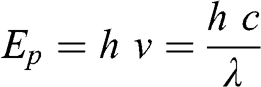
The Sun consists of about three-quarters of hydrogen and one quarter of helium. Helium is formed by a fusion reaction between hydrogen atoms, which generates energy. This energy escapes from the Sun as electromagnetic radiation. This solar radiation comprises photons that carry energy, which is a function of wavelength. The radiation frequency, ν(s−1), associated with a photon is related to the wavelength of the radiation, λ (m), via the speed of light, c (m s−1):
 (5.1)
(5.1) The energy of a photon, Ep (J), of wavelength λ is:
 (5.2)
(5.2) where h is the Planck constant (h = 6.626 × 10⁻³⁴ J s). Therefore, the energy of a photon increases as its wavelength decreases.
The electromagnetic spectrum covers a wide range of wavelengths. Visible light ranges from about 400 to 700 nm, with violet light at about 400 nm, blue light at about 450 nm, green light at about 550 nm, and red light at about 650 nm. Below 400 nm is ultraviolet (UV) radiation. At wavelengths far below UV radiation are X rays (from about 0.001 to 10 nm) and gamma rays (from about 0.1 to 1 pm). Above 700 nm is infrared (IR) radiation. At greater wavelengths are radar wavelengths (from about 1 mm to 1 m), as well as television and radio wavelengths. Since the energy of radiation decreases with increasing wavelength, UV radiation has more energy than IR radiation.
Solar radiation covers a range of wavelengths. The Sun emits radiation, which corresponds approximately to that of a black body at a temperature of about 5,800 K. In comparison, IR radiation reemitted by the Earth corresponds to that of a black body at about 300 K. (The term “black body” corresponds to the assumption that this body absorbs all radiation completely and does not reflect it; however, the temperature of this body leads to radiation that is maximum at a wavelength that depends on the temperature of this body and, therefore, it is not actually black.)
Solar radiation is partially scattered and absorbed by gases present in the atmosphere and, consequently, some of the radiation does not reach the Earth’s surface. Oxygen and nitrogen molecules absorb solar radiation below 100 nm. Between 100 and 200 nm, molecular oxygen strongly absorbs solar radiation. Between 200 and 280 nm, ozone (a product of the oxygen photolysis, see Chapter 7) also absorbs radiation very effectively. Therefore, solar radiation reaching the Earth’s surface corresponds mostly to wavelengths greater than 280 nm. Figure 5.1 shows the solar radiation spectrum at the top of the atmosphere, as well as at sea level, i.e., after scattering and absorption by atmospheric gases. Scattering of solar radiation by cloud droplets is also taken into account in this figure.
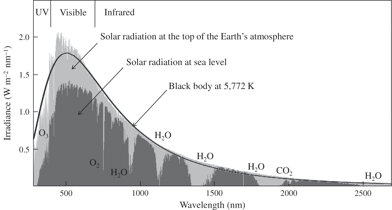
Figure 5.1. Solar radiation spectrum reaching the Earth. The solid black line corresponds to the theoretical irradiance of a black body at 5,772 K located at the distance of the Sun and calculated at the top of the Earth’s atmosphere. The light gray shaded area corresponds to solar radiation at the top of the Earth’s atmosphere and the dark gray shaded area corresponds to solar radiation reaching the Earth’s surface after scattering and absorption by atmospheric gases and reflection by clouds. Gases absorbing radiation are indicated at their major absorption wavelengths.
Triatomic gases such as water vapor (H2O), carbon dioxide (CO2), and ozone (O3) form dipoles, which interact with the electromagnetic radiation at IR wavelengths. These molecules are, therefore, greenhouse gases, because they do not absorb much solar radiation, which is mostly in the UV and visible light range (except ozone, which absorbs some UV light, see Chapter 7), but they absorb IR light, which is emitted by the Earth. For example, CO2 shows its maximum absorption at about 15 μm, which corresponds to the wavelength range near the maximum IR emission by the Earth’s surface.
5.1.2 Radiance and Irradiance
Radiance (or intensity), I, represents the radiative energy per unit time (W or J s−1) per unit surface area (m−2), and per unit solid angle (sr−1). It can be integrated over all wavelengths (W m−2 sr−1) or expressed monochromatically (spectral radiance) per unit wavelength (W m−2 sr−1 nm−1).
Irradiance, Ee, represents the radiative energy flux going through a surface. Therefore, it corresponds to the component of the radiance that is perpendicular to the surface and integrated over all solid angles of the hemisphere corresponding to the side of the surface where the source is located. If the angle between the direction of the radiation and the direction perpendicular to the surface is θr:
 (5.3)
(5.3) where Ω is the direction of the incoming radiation. Irradiance may be integrated over all wavelengths (W m−2) or expressed monochromatically per unit wavelength (monochromatic or spectral irradiance in W m−2 nm−1).
5.1.3 Radiative Budget of the Earth’s Atmosphere
The spectral radiance of a black body is governed by Planck’s law:
 (5.4)
(5.4) where kB is the Boltzmann constant (1.381 × 10⁻²³ J K−1) and T is the temperature in K. Therefore, radiance increases as the temperature of the black body increases, for all wavelengths. The wavelength corresponding to the maximum radiance, λmax, is approximately given by Wien’s law:
 (5.5)
(5.5) where λ is in nm and T in K. Therefore, the greater the temperature, the smaller the wavelength corresponding to the maximum radiance. The estimation of the effective temperature of the Sun’s surface (photosphere) is on the order of 5,770 to 5,780 K. For a temperature of 5,772 K (NASA, 2017), the wavelength corresponding to the maximum radiance of the Sun is calculated as follows:

This wavelength corresponds to a blue-green light. However, blue light is preferentially scattered by the molecules of the Earth’s atmosphere and the Sun’s appearance is yellow or even red when the Sun is near the horizon (see the discussion of atmospheric visibility in Section 5.2). Outside the atmosphere, the Sun’s appearance is white because its radiation spectrum covers all visible wavelengths. The full spectrum of the colors of solar radiation is clearly visible in a rainbow, because the water droplets decompose this radiation spectrum due to refraction of the incoming radiation, which modifies the direction of the photon trajectories depending on their wavelength.
The Stefan-Boltzmann law relates the irradiance of a black body to its temperature. It is derived from Planck’s law by integrating over all wavelengths:
where σSB is the Stefan-Boltzmann constant (5.67 × 10⁻⁸ W m−2 K−4).
Thus, the irradiance of the Sun at its source is:
At the distance of the Earth’s orbit, this irradiance is smaller, since it has been dispersed over a greater sphere, which has a radius equal to the distance between the Sun and the Earth. This irradiance of solar radiation at the Earth’s orbit is called the solar constant, ES:
 (5.7)
(5.7) Thus:
where the distances are expressed in km. This value corresponds to that obtained by irradiance measurements performed via the Solar Radiation and Climate Experiment (SORCE) NASA satellite (Kopp and Lean, 2011). The radiative energy intercepted by the Earth corresponds to the radiative energy flux (irradiance) integrated over the Earth’s cross-section, i.e., Es π rT2, where rT is the Earth’s radius (6,371 km). Therefore, the average radiative flux reaching the top of the Earth’s atmosphere is equal to this value divided by the Earth’s surface area, π rT2 ES / (4 π rT2), i.e., ES / 4, which corresponds to about 340 W m−2.
However, part of the solar radiation is reflected toward space by clouds, atmospheric particles, and the Earth’s surface. This fraction, called albedo, is on the order of 30 %. Therefore, the solar radiative flux absorbed by the Earth and its atmosphere, Ee,E, is estimated to be on average about 235 W m−2 and about 105 W m−2 are reflected toward space.
If the Earth is considered to be a black body and if one assumes that the radiative flux received by the Earth (235 W m−2) is at equilibrium with that reemitted by the Earth, then the temperature at the Earth’s surface is estimated from the Stefan-Boltzmann law:
 (5.8)
(5.8) The average temperature at the Earth’s surface is actually greater, since it is on average 288 K (15 °C). The difference between these two temperatures is due mostly to the absorption of part of the radiative energy reemitted by the Earth by some gases present in the Earth’s atmosphere. These gases are called greenhouse gases (GHG). The radiative budget of the Earth must, therefore, take into account the effect of these GHG, as well as some other important processes.
First, the radiative energy reflected to space may be decomposed into a fraction reflected by the atmosphere (clouds and particles), which is about 75 W m−2, and a fraction reflected by the Earth’s surface (in particular by snow and ice, which have a strong albedo), which is about 30 W m−2. The fraction absorbed may be decomposed into a fraction absorbed by the atmosphere (mostly in the UV), which is 67 W m−2, and a fraction absorbed by the Earth’s surface, which is 168 W m−2.
Radiation emitted by the Earth is located in the IR range. Therefore, this radiation is partially absorbed by GHG (see Figure 5.2). Natural GHG are water vapor (H2O) and CO2. In addition, anthropogenic activities lead to greater CO2 atmospheric concentrations, since it is a product of combustion. Other GHG that are due to anthropogenic activities include methane (CH4), nitrous oxide (N2O), and ozone (O3). The relative contributions of these GHG to the absorption of IR radiation are presented in Chapter 14. All GHG absorb about 350 W m−2. This amount corresponds to about 90 % of the IR radiative flux emitted by the Earth’s surface, which is 390 W m−2; therefore, 40 W m−2 are directly emitted into space through a window of the IR spectrum where there is little absorption by GHG.

Figure 5.2. Radiation spectrum emitted by the Earth in the infrared with the absorption bands of some greenhouse gases (CO2, H2O, CH4, and O3). The solid line corresponds to a simulation with the MODTRAN radiative transfer model (Spectral Sciences, Inc. and U.S. Air Force Research Laboratory; http://modtran.spectral.com) for a standard U.S. atmosphere at an altitude of 50 km. The dashed line corresponds to the radiation flux of a black body at 288 K at the same altitude. The atmospheric windows through which the Earth’s radiation flux escapes to space appear clearly between 8 and 9 μm and between 11 and 13 μm.
In addition, the Earth’s surface emits heat (1) via water evaporation, which releases heat during its subsequent condensation in the atmosphere leading to cloud and fog formation (latent heat flux), and (2) via heat fluxes due to atmospheric turbulence (sensible heat flux); see Chapter 4 for the description of the physical processes corresponding to these heat fluxes. These two fluxes correspond to about 102 W m−2 (78 and 24 W m−2, respectively).
Therefore, the total amount of energy absorbed by the atmosphere is 519 W m−2, which includes 67 W m−2 via absorption in the UV, 350 W m−2 via absorption in the IR, and 102 W m−2 via the latent and sensible heat fluxes. At equilibrium, the atmosphere reemits this energy: 62 % (324 W m−2) toward the Earth’s surface and 38 % (195 W m−2) toward space. The fact that the most important fraction is emitted toward the Earth’s surface results from the vertical distribution of the atmospheric density, which is greater near the Earth’s surface.
In summary, the radiative flux at the top of the atmosphere is 340 W m−2, the atmosphere absorbs and reemits 519 W m−2, and the Earth receives and reemits 522 W m−2, of which 30 W m−2 correspond to the Earth’s albedo. Table 5.1 summarizes the different components of these energy fluxes in terms of their sources and associated processes.
Table 5.1. Summary of the energy balance of the Earth and its atmosphere (W m−2).
| Earth | Absorbed energy (source) | Emitted energy (process) |
| 168 (Sun; absorption) | 390 (IR) | |
| 324 (GHG) | 102 (heat) | |
| Budget for the Earth* | 492 | 492 |
| Atmosphere | Absorbed energy (source) | Emitted energy (process) |
| 67 (Sun) | 324 (IR toward the Earth) | |
| 350 (Earth; IR) | 195 (IR toward space) | |
| 102 (Earth; heat) | ||
| Budget for the atmosphere | 519 | 519 |
| Top of the atmosphere | Incoming energy (source) | Outgoing energy (source) |
| 340 (Sun) | 75 (cloud albedo) | |
| 30 (Earth’s albedo) | ||
| 195 (IR from GHG) | ||
| 40 (IR form the Earth) | ||
| Budget at the top of the atmosphere | 340 | 340 |
* In addition, 30 W m−2 are directly reflected by the Earth (albedo).
The radiative energy reemitted by the Earth’s surface as IR radiation is 390 W m−2. Applying the black body formula for this irradiance (see Equation 5.8) leads to a temperature of 288 K (i.e., 15 °C), which is consistent with the mean temperature at the Earth’s surface. The wavelength corresponding to the maximum radiation emitted by the Earth may be calculated by Wien’s law (Equation 5.5): it is 10 μm, which corresponds to the infrared range.
More solar radiation is absorbed at the equator than at the poles, because of the zenith angle (i.e., the angle between the direction of the direct solar radiation and the direction perpendicular to the surface). The Earth reemits also more IR radiation at the low latitudes (tropical regions) than at the high latitudes (polar regions). However, the gradient from the equator to the poles is less pronounced for reemission than for absorption. This difference is due (1) to a greater reflectance (i.e., greater albedo) of the Earth’s surface at the poles than in the tropical regions and (2) to the presence of more water vapor (greater humidity) in the tropical regions and the associated clouds and latent heat release aloft. The energy budget leads, therefore, to a net gain in the tropical regions and a net loss in the polar regions (see Figure 5.3). These energy differences must, therefore, lead to a transfer of energy from the equator to the poles, in order to maintain global equilibrium for the Earth. This energy transfer corresponds to the Hadley cells in the tropical and sub-tropical regions and the polar cells near the poles. In addition, the ocean currents transfer also some heat from the equator toward regions at higher latitudes. Finally, the water vapor emitted in the tropical regions is transported toward mid-latitude regions, which corresponds to a latent heat flux from the low toward the higher latitudes.

Figure 5.3. Schematic representation of the meridional profile of the Earth’s energy budget.
5.2 Atmospheric Visibility
Here, the absorption and scattering of atmospheric radiation by molecules and particles are briefly described. Next, the calculation of the visual range (i.e., the distance at which the human eye can see an object in the atmosphere) is presented. Finally, some examples of the effect of some air pollutants in terms of discoloration of the atmosphere are provided.
5.2.1 Absorption of Atmospheric Radiation
Some gases and particles absorb atmospheric radiation. The amount of light absorbed is proportional to the absorption efficiency of the absorbing species, ka (m2 g−1), its concentration, C (g m−3), and the distance traveled by the radiation, dx. The absorption coefficient (m−1) is defined as the product of the absorption efficiency and the concentration:
Assuming a uniform concentration of the absorbing species, the change in the radiance may be calculated as a function of the distance traveled by the radiation according to Beer-Lambert’s law:
where dI is the amount of radiance absorbed over the distance dx. Integrating from 0 to x:
where I0 is the initial radiance at x = 0. In the case of an object, it is called the intrinsic radiance.
5.2.2 Scattering of Atmospheric Radiation
Atmospheric radiation is scattered by gas molecules, particles, and droplets (for example, cloud and fog droplets). Mie theory describes the scattering of radiation by molecules and particles. For gas molecules and ultrafine particles (<100 nm), the wavelengths of the visible range are greater than the molecule or particle size. This range is called the Rayleigh scattering regime, where radiation is scattered as a function of wavelength following a λ−4 function. Therefore, molecules and ultrafine particles scatter preferentially blue light (between 400 and 450 nm) compared to the other colors of the visible spectrum and scatter red light the least. A clear sky during daytime, looking away from the Sun, represents this scattered radiation and, therefore, appears blue. At sunset or sunrise, solar radiation along the line of sight of an observer looking at the horizon travels through a maximum distance of the atmosphere (almost tangential to the Earth’s surface) and red light, which is the least affected by scattering, dominates and gives the red appearance of sunsets and sunrises.
Atmospheric radiation is not scattered in an isotropic manner, but is scattered differently in various directions. The anisotropy of scattered radiation is represented mathematically by the phase function, p(Ω’ —› Ω), where Ω’ and Ω are the directions of the incoming radiation and scattered radiation, respectively. In the Rayleigh regime, scattering occurs mostly along the incoming radiation direction, in equal amounts forward and backward. The amount of radiation scattered in the other directions is less and it is minimum in the direction perpendicular to the incoming radiation (half the amount scattered in the direction of the incoming radiation).
For particles, Mie theory predicts phase functions that correspond to forward scattering dominating for coarse particles (i.e., those particles greater in diameter than 2.5 μm). Actually, forward scattering is already dominant for particles with a diameter greater than 0.5 μm. For example, in presence of fog, the intensity of a light is preferentially scattered forward along the direction of the incoming light.
Beer-Lambert’s law may be applied to scattering to calculate the fraction of radiation that is not scattered out of the line of sight. The scattering coefficient, bs, is defined as the product of the scattering efficiency, ks, and the concentration of the scattering species (molecule or particle):
where dI is the amount of radiation scattered along the distance dx. Integrating from 0 to x:
In the general case where both absorption and scattering take place, an extinction coefficient, be, may be defined, which corresponds to the sum of both phenomena:
Beer-Lambert’s law is then written as follows:
5.2.3 Optical Thickness
Optical thickness (also called optical depth), τ, is defined as the integral value of the extinction coefficient along a given distance. For example, in the case of a measurement performed by a satellite-borne instrument, it is the value integrated over the atmospheric height between the Earth’s surface and the satellite:
 (5.16)
 The optical thickness is dimensionless. The extinction coefficient, be, is placed within the integral because it may vary with distance (here altitude), for example, if the concentrations of the absorbing and/or scattering species vary with distance.
5.2.4 Visual Range
The visual range is the utmost distance at which an observer can perceive a black object (see Figure 5.4). The criterion of a 2 % contrast between the object and the background is typically used as the perception threshold for the human eye. Contrast, Co, is defined as the relative difference between the background radiance, Ib, and that of the object, Io:
 (5.17)
 For a black object, Io(x = 0) = 0 (since it does not reflect any light) and its intrinsic contrast, i.e., at x = 0, is 1.

Figure 5.4. Schematic representation of visible atmospheric radiation between an object and an observer. See text for the definitions of the various terms.
Over a distance dx along the line of sight between the object and the observer, the radiance increases due to scattering of background light into the line of sight and the radiance of the object decreases due to light extinction along the line of sight. According to the radiative transfer equation (Chandrasekhar, 1960; Goody et Yung, 1989), the radiance from an object, Io(Ω, 0), reaching the observer at a distance x and in a direction Ω, is calculated as follows:
 (5.18)
 where τx is the optical thickness, ωa is the albedo, and p(Ω’ —› Ω,τ’) is the phase function. The first term on the right-hand side of the equation represents the decrease in the radiance due to particles and gases that absorb and scatter light, and the second term represents the radiance added by scattering of the background light into the line of sight of the observer. At x = 0, the solution corresponds to the intrinsic radiance of the object, Io(Ω, 0), and, when x —› ∞ , the solution tends toward the background radiance, Ib, (i.e., the object is no longer perceptible). This integral equation may be solved numerically in the general case. For the simple case where the scattering and absorption coefficients are uniform between the object and the observer, this equation may be written as follows:
 (5.19)
 To calculate the contrast, the radiance originating from the object and the background radiance (i.e., at the horizon near the object) must be calculated. The change in the radiance coming from the object due to light scattering is obtained from Equation 5.19. By derivation, the solution for an incremental distance dx is as follows:
This equation corresponds to the difference between the radiance added and that subtracted along the line of sight. By definition, the background radiance is spatially uniform, i.e., Ib(x) = Ib, a constant value. The change in the contrast may be calculated along the distance dx:
 (5.21)
 According to the relationship for dIo(x), i.e., Equation 5.20:
 (5.22)
 The ratio on the right-hand side is equal to bs Co(x). Therefore, the contrast follows Beer-Lambert’s law:
Integrating from 0 to x:
where Co0 is the intrinsic contrast of the object, often chosen to be 1 by default. If the perception threshold criterion is chosen to be 2 % (Co / Co0 = 0.02) at 550 nm (i.e., the wavelength at which perception is maximum for the human eye), the visual range, VR, which is the maximum distance at which an object can be perceived, is given by the following equation:
Solving for VR leads to the Koschmieder relationship (1924):
 (5.26)
 Several assumptions are implicit in this equation:
– The atmosphere is spatially uniform in terms of light scattering.
– The background radiance is the same at the object and at the observer location.
– The observed object is black and thus has an intrinsic contrast of 1 (i.e., at x = 0).
– The minimum contrast that is perceptible is 2 % (a value up to 5 % is sometimes used).
– The Earth’s curvature is neglected (i.e., this relationship cannot be applied to atmospheres approaching Rayleigh scattering, see example).
– The extinction coefficient represents only scattering and does not include absorption (see discussion later in this section).
The relationship for the change in contrast as a function of distance is different for light absorption. In the case of absorption, both the background radiance and that of the object decrease similarly with distance in the case where absorption occurs between the object and the observer:
and:
Thus, the difference between the two radiances decreases according to Beer-Lambert’s law. Therefore, the contrast does not follow Beer-Lambert’s law, but remains constant in the case of absorption. If one considers both scattering and absorption, the change of the radiances with distance may be written as follows:
and:
The solutions to these differential equations are as follows:
Thus:
The contrast of the object with respect to the background is not affected by the absorption of light between the object and the observer. On the other hand, the perception of the object becomes more difficult because the transfer of its radiance decreases due to absorption. In addition, if the air pollution extends beyond the distance at which the object is located, the background radiance will be affected more by absorption than it was in the previous calculation, where it was assumed that absorption occurs only between the object and the observer. Absorption will then decrease the background radiance and make it darker. The effect on the contrast will then depend on the color of the object compared to that of the background. An object that is darker than the background will have a lesser contrast and an object that is brighter than the background will have a greater contrast. In the case of a black object observed against a clear sky background, air pollution extending beyond the object will decrease its contrast. However, it is not possible to calculate this change in contrast simply and it is necessary to perform a radiative transfer calculation using a numerical model (see Section 5.3).
The assumption that is generally made in the empirical formulas used to calculate visual range is that the Koschmieder relationship applies to the extinction coefficient (i.e., both scattering and absorption). Since the extinction coefficient is generally dominated by scattering rather than by absorption, this approximation is considered acceptable. However, it is not strictly correct:
 (5.34)
 For a pristine atmosphere, scattering follows the Rayleigh regime and there is no absorption. The scattering coefficient can be calculated according to the following relationship:
 (5.35)
 where P is the atmospheric pressure in atm, T is the temperature in K, and bRay,ref(λ) is the Rayleigh scattering coefficient at 1 atm and 0 °C. Some values for the visible range are provided in Table 5.2.
Table 5.2. Rayleigh scattering coefficient at 1 atm and 0 °C as a function of wavelength in the visible range (1 Mm = 106 m).
| Wavelength (nm) | bRay,ref(λ) (Mm−1) |
|---|---|
| 400 | 45.40 |
| 450 | 27.89 |
| 500 | 18.10 |
| 550 | 12.26 |
| 600 | 8.604 |
| 650 | 6.217 |
| 700 | 4.605 |
At 1 atm and 15 °C, for a wavelength in the middle of the visible range, i.e., 550 nm (green light):
bRay = 11.6 Mm−1
This simple formula does not take into account the fact that the refraction index depends on temperature. Nevertheless, it is a good approximation at ambient temperatures (for example, 1 % error at 15 °C).
The calculation of the extinction coefficient requires knowing the concentrations, chemical composition, and size distribution of atmospheric particles and, to a lesser extent, the concentration of NO2 (which absorbs light in the visible range). In the absence of detailed information on particle size distribution, empirical formulas based on the chemical composition of particulate matter and atmospheric humidity may be used (humidity affects the size of hygroscopic particles, see Chapter 9). For example, the formula used by the U.S. National Park Service (EPA, 2003) is as follows:
 (5.36)
 This equation corresponds to a wavelength of 550 nm (green light), which is in the middle of the visible range. Units are Mm−1 (per megameter) for the extinction and scattering coefficients, μg m−3 for concentrations, and m2 g−1 for the scattering and absorption efficiencies. The numerical values represent the scattering efficiencies of various components of atmospheric particulate matter and the absorption efficiency of black carbon. The first five terms correspond to fine particles (i.e., those particles with a diameter less than 2.5 μm) and the size distribution of those particles is supposed to be lognormal with a mean diameter of 0.3 μm and a standard deviation of 2 (see Chapter 9 for a description of the lognormal distribution). The function fas(RH) represents the growth of inorganic fine particles via absorption of water as atmospheric humidity increases (i.e., hygroscopicity); a larger particle is more efficient at scattering light. This function was obtained by calculating the size of an ammonium sulfate particle as a function of relative humidity (RH). The particle size is an average value between the deliquescence and efflorescence particle sizes (see Chapter 9). For example, fas(RH) is equal to 1 (dry particles) at very low humidity (<30 %), but is equal to 1.5 at 60 %, 2 at 70 %, 2.5 at 80 %, 3 at 85 %, 4 at 90 %, and 10 at 95 % relative humidity. Organic particulate matter is assumed to be hydrophobic and, therefore, its scattering efficiency does not depend on humidity. Black carbon is also hydrophobic; in any case, its absorption efficiency depends on its concentration and not on particle size. The size distributions of coarse soil dust and sea salt particles are assumed to be lognormal, with a mean diameter of 5 μm and a standard deviation of 2. The function fss(RH) represents the hygroscopic growth of sea salt particles; it differs from that used for ammonium sulfate particles. This type of formula is empirical (i.e., it involves various assumptions on particle size distributions, hygroscopic growth, etc.) and there are other similar formulas available to estimate the extinction coefficient for polluted atmospheres.
The haze index, DHI, which is expressed in deciview (dv), was introduced to quantify atmospheric visibility (Pitchford and Malm, 1994). It is defined by the following equation, by analogy with the decibel unit for sound:
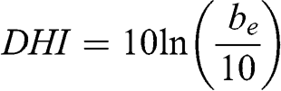 (5.37)
 where be is expressed in Mm−1. A change of 1 dv corresponds to a change of about 10 % in the extinction coefficient and, therefore, in the visual range (10.52 % more precisely). Given that the scattering coefficient for a Rayleigh atmosphere is about 10 Mm−1, such an atmosphere has a haze index of about 0 dv. A visual range of 1 km corresponds to 60 dv, 10 km to 37 dv, and 100 km to 13.6 dv. The advantage of the haze index is that it changes linearly in terms of perception by the human eye.
Example: Calculation of the visual range for a Rayleigh atmosphere (pristine air)
According to Equation 5.35, the Rayleigh scattering coefficient at 550 nm is 11.6 Mm−1 at 1 atm and 15 °C. Therefore, in an atmosphere without any particles, the visual range given by the Koschmieder relationship (Equation 5.26) is:
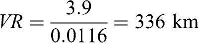
Actually, such a visual range should take into account the curvature of the Earth and should integrate the Rayleigh scattering coefficient along an optical path, because this scattering coefficient decreases with altitude. Indeed, looking toward the horizon over a distance of 336 km leads to an altitude located well above sea level at the distance of the visual range. The radius of the Earth is 6,371 km; the angle θo between the direction from the center of the Earth to the observer and that from the center of the Earth to the visual range virtual location may be calculated as follows:
Therefore, the distance from the center of the Earth to the location corresponding to the visual range is:
Therefore, the corresponding altitude of that location is (6,380 – 6,371) = 9 km. This altitude is greater than the highest Himalayan mountain tops. Since the Rayleigh scattering coefficient decreases with atmospheric pressure, the visual range would actually be greater. In any case, no fixed object is located at such an altitude along the sight path of the observer and the concept of visual range seems then difficult to apply.
Example: Estimation of the visual range during an air pollution episode in Paris, France
During the air pollution episode of March 2014 (see Chapter 9), the particulate matter concentrations were measured by the Laboratoire des sciences du climat et de l’environnement (LSCE) and by the Institut national de l’environnement et des risques industriels (Ineris) in Saclay, a suburban area located southwest of Paris. On March14 at 10 a.m., these concentrations were approximately as follows (the background air pollution during this episode was fairly uniform and it seems appropriate to use those measurements to represent air pollution over the Paris region):
– Ammonium sulfate concentration: 9 μg m−3
– Ammonium nitrate concentration: 45 μg m−3
– Organic particulate matter concentration: 18 μg m−3
– Black carbon concentration: 1 μg m−3
– Sea salt concentration: negligible
– Soil dust concentration: no available measurements (zero concentration by default)
– Coarse particulate matter concentration: ~70 μg m−3 (estimation based on PM10 measurements performed by Airparif; see Chapter 9)
A temperature of 15 °C and a relative humidity of 60 % are assumed; thus f(RH) = 1.5.
The empirical formula given by Equation 5.36 is used the calculate the extinction coefficient:

Thus: be = 379 Mm−1
Absorption contributes only 3 % to be, which is dominated by light scattering. Applying the Koschmieder relationship (Equation 5.34) to estimate visual range:
This distance corresponds approximately to the distance between Notre-Dame Cathedral and the Grande Arche in the Défense business district located west of Paris or the distance between Saint-Germain-en-Laye Castle and the Défense business district. This result implies that during such an air pollution episode, it would not be possible to see the Défense business district from Notre-Dame in downtown Paris or from Saint-Germain-en-Laye (actually, since the Grande Arche in the Défense business district is not black, it will be even less visible than estimated by the Koschmieder relationship). The corresponding deciview haze index is:
5.2.5 Colors of Air Pollution
Plumes emitted from tall stacks or from tail pipes may have different colors depending on the pollutants emitted or, in the case of particles, the relative positions of the observer, the Sun, and the plume.
Some gases absorb radiation and, if this absorption occurs in the visible range, the color of the gas will correspond to the wavelengths that are not being absorbed. The main example in air pollution is nitrogen dioxide (NO2), which absorbs radiation in the blue, violet, and UV (Burkholder et al., 2015). Thus, its color results from wavelengths ranging from the green to the red wavelengths and a NO2 plume will appear orange-brown.
Black-carbon particles absorb strongly and, therefore, they appear black, since almost no light is scattered by those particles (Bond and Bergstrom, 2006). For example, some diesel vehicles without any particle filter may lead to a small black puff of black carbon when starting or accelerating.
Ultrafine particles have sizes that are near those of molecules and they scatter radiation preferentially at small wavelengths, i.e., in the visible range, at blue and violet wavelengths. Therefore, a large concentration of ultrafine particles leads to a bluish color of the air. This phenomenon occurs in areas with pristine air where there is a lot of vegetation. Vegetation leads to emissions of volatile organic compounds, terpenes and terpenoids, which, after oxidation in the air, form semi-volatile organic compounds. In the absence of large concentrations of other particles, these compounds nucleate to form new ultrafine particles (see Chapter 9). This phenomenon has led to several terms on various continents:
– The Blue Ridge Mountains in Virginia, United States
– The Blue Mountains in New South Wales, Australia
– The Blue Mountains in Jamaica, Caribbean
– And perhaps also the blue line of the Vosges Mountains, France
Fine and coarse particles and water droplets scatter all wavelengths of the visible spectrum and they appear gray. However, this appearance may vary from white to black depending on the particle/droplet concentration and the angle between the solar radiation direction, the plume, and the line of sight of the observer.
5.3 Numerical Modeling of Atmospheric Radiation
Numerical modeling of atmospheric radiation is needed in air pollution models to calculate the kinetics of photochemical reactions (see Chapter 7). The assumption of a plane atmosphere is generally made to simplify the geometry of the radiative fluxes. The simplest approach consists in considering only two directions for the radiative transfer, upward and downward. This simplification allows one to obtain a simple numerical solution of the radiative transfer equation. The adding and doubling method (or one of its variants) may be used to obtain the numerical solution. If standard atmospheric conditions are used, the calculation of the atmospheric radiative fluxes may be performed as a preprocessing step to an air pollution simulation. It can then be performed using a large number of wavelengths, and the photolytic kinetic constants can be tabulated for future use during the air pollution simulations. However, this approach only applies to optically thin atmospheric conditions, i.e., in cases where the presence of particles and droplets can be neglected.
Since atmospheric radiation may be significantly affected by the presence of clouds and particles that scatter radiation (and in the case where black carbon absorbs it) and since clouds and particle concentrations vary spatially and temporally during an air pollution simulation, it is preferable to perform the radiative transfer calculation online, i.e., concurrently with the air pollution simulation, in order to calculate the photolytic rates based on the more representative atmospheric conditions. Several algorithms have been developed to perform such calculations. For example, the FAST-J algorithm can perform this type of calculation for atmospheres with cloud layers and particles (Wild et al., 2000). FAST-J uses a two-dimensional geometry with eight directions for radiation scattering and a spectral resolution of up to 18 wavelengths.
Modeling the degradation of atmospheric visibility is generally limited to the calculation of the extinction coefficient to assess regional haze (see Section 5.2.4). Nevertheless, models of atmospheric visibility have been developed to calculate the visual impacts (contrast and color) of industrial stack plumes. This type of modeling is significantly more difficult than modeling regional haze, because the position of the observer with respect to the plume and the Sun must be taken into account, in order to calculate light scattering by the particles present in the plume correctly. Atmospheric visibility models give satisfactory results for plumes that absorb the atmospheric light; for example, a nitrogen dioxide plume emitted from a power plant (White et al., 1985). However, their performance is less satisfactory in the case of light-scattering plumes (i.e., particle-laden plumes) (White et al., 1986). The reason is that the phase functions depend strongly on the particle size distribution of the particles or droplets and the simulation of multiple scattering with complex geometries is challenging. If the particle/droplet size distribution is known, numerical methods such as discrete ordinate methods may be used to discretize the radiative transfer equation in different directions over finite volumes. Monte-Carlo methods may also be used to obtain better accuracy; such methods solve the radiative transfer equation with a large array of calculations representing the effect of multiple scattering on the paths of photons that are sampled randomly (e.g., Thomas and Stamnes, 1999). However, Monte-Carlo methods are computationally demanding and they have not been used operationally in air pollution modeling.
Problems
Problem 5.1 Absorption of atmospheric radiation
The absorption efficiency of visible light by black carbon is assumed to be 10 m2 per g of black carbon. The black-carbon atmospheric concentration in Paris during an air pollution episode is given to be 4 μg m−3. In Paris, an observer is looking at Arc de Triomphe from Place de la Concorde; the distance between these two locations along Avenue des Champs-Élysées is 2 km. Calculate the fraction of light that is absorbed by black carbon along this sight path using Beer-Lambert’s law.
Problem 5.2 Visual range
During a spring air pollution episode in Paris, scattering dominates over absorption to degrade atmospheric visibility (bs = 400 Mm−1). Instead of applying the Koschmieder relationship to calculate the visual range, as done in the example above, it is assumed here that a monument will be perceptible only when its contrast is 5 % (i.e., instead of 2 %).
a. Calculate the distance at which this monument will no longer be visible.
b. By which amount should the ammonium nitrate particulate concentration be reduced in order to double the visual range? One assumes here that the initial ammonium nitrate concentration is 50 μg m−3.