Abstract
Atmospheric dispersion is a very important process in air pollution. The use of tall stacks to minimize the impacts of air pollutant emissions reflected the saying that “the solution to pollution is dilution.” Although this saying turned out to be wrong for several reasons, including the cumulative effect of a large number of individual sources and the formation of secondary pollutants at large regional scales, atmospheric dispersion is nevertheless one of the key processes that govern air pollution levels. This chapter presents the fundamental processes of atmospheric dispersion, their theoretical basis, as well as the advantages and shortcomings of different types of atmospheric dispersion models.
Atmospheric dispersion is a very important process in air pollution. The use of tall stacks to minimize the impacts of air pollutant emissions reflected the saying that “the solution to pollution is dilution.” Although this saying turned out to be wrong for several reasons, including the cumulative effect of a large number of individual sources and the formation of secondary pollutants at large regional scales, atmospheric dispersion is nevertheless one of the key processes that govern air pollution levels. This chapter presents the fundamental processes of atmospheric dispersion, their theoretical basis, as well as the advantages and shortcomings of different types of atmospheric dispersion models.
6.1 General Considerations on Atmospheric Dispersion
Pollutants are dispersed, and therefore diluted, in the atmosphere as a result of turbulence. This turbulence covers a wide range of spatial scales, including large-scale eddies, smaller eddies, and so on until the dispersion of kinetic energy at the molecular scale. Lewis Fry Richardson (1881–1953), an English physicist, summarized this cascade of processes in a more poetic fashion:
“Big whirls have little whirls that feed on their velocity,
and little whirls have lesser whirls and so on to viscosity.”
Since it is not possible to represent turbulence in a mathematical deterministic manner, it is necessary to introduce approximate representations of the main processes involved. Because of the presence of the Earth’s surface, which creates an anisotropy in the lower layers of the atmosphere, it is appropriate to differentiate between turbulence in the vertical and horizontal directions.
Vertical turbulence results from processes mentioned in Chapter 4, which include mechanical turbulence and thermal turbulence. The latter depends strongly on the thermal structure of the planetary boundary layer (PBL); it is very large when the atmosphere is unstable and weak when the atmosphere is stable. Convection phenomena, which occur in the PBL as well as in the free troposphere, mix also air parcels (and, therefore, air pollutants) in the vertical direction, but they typically correspond to coherent motions and, therefore, are not treated in detail here.
Horizontal turbulence may be created by mechanical processes in the PBL, as well as by thermal processes. It is more challenging to parameterize the relevant physical processes, compared to those governing vertical motions. Therefore, its mathematical modeling can be difficult, particularly at very large spatial scales.
Turbulent processes can be addressed either through a lagrangian or an eulerian approach. In the lagrangian approach, one uses a reference system that moves with the mean wind and turbulent motions are studied with respect to that moving reference system. Therefore, one refers to relative turbulent diffusion, because it is relative to this reference system. Thus, the meandering of a plume, which may result from large-scale motions affecting the reference system, is not included. Relative diffusion corresponds to the instantaneous plume size, because averaging the plume size over time will correspond to including some of the plume meandering in the plume size. In the eulerian approach, the ensemble of turbulent motions is considered with respect to a fixed reference system. Therefore, one refers to absolute turbulent diffusion. Both approaches become equivalent when the lagrangian approach covers the full range of the turbulent eddies.
6.2 Lagrangian Representation of Turbulence
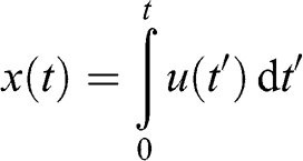
In the lagrangian representation of turbulence, one follows the statistical evolution of the distance between two particles (or molecules) emitted from the same source (Csanady, 1973). If a particle is present at the location x’ at time t = 0, its random motion may be represented with the probability density p(x − x’, t) such that p(x − x’, t) dx is the probability that the motion of the particle during time t leads to its arrival in a space dx centered at the location x. Then, the concentration of particles present at time t at the location x (i.e., the mass of particles within a volume dx) is as follows:
where S0 is the mass of particles emitted at time 0 at the location x’. The assumption of a random turbulent diffusion process leads to a gaussian distribution of the particle concentrations with a standard deviation σ and its maximum at the source location x’. In three dimensions, the standard deviation of the distribution of particles undergoing turbulent diffusion may be defined in one direction (here x) for the entire particle population as follows (assuming that the source is at x’ = y’ = z’ = 0):
 (6.2)
(6.2) Therefore, the standard deviation of the particle distribution in one direction is equivalent to the root mean square of the motions of the particles in that direction. If turbulence is uniform and isotropic, then: σx = σy = σz = σ. The distance traveled by a particle at the speed u during time t is:
 (6.3)
(6.3) Therefore, the change in the square of the distance traveled as a function of time is as follows:
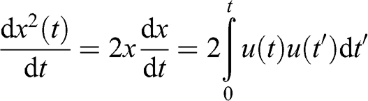 (6.4)
(6.4) Taking the ensemble average for both sides of the equation:
 (6.5)
(6.5) The autocorrelation between the velocities of two particles at times t and t’ = t + τ□ is as follows:
 (6.6)
(6.6) Therefore, the change of the standard deviation as a function of time is written as follows (dt’ becomes dτL):
 (6.7)
(6.7) This expression is known as Taylor’s theorem (1922) (Geoffrey Ingram Taylor was a British physicist and mathematician). After integration:
 (6.8)
(6.8) Integrating by parts provides the solution for the square of the standard deviation of the distribution of particles for a steady-state dispersion process:
 (6.9)
(6.9) Thus:
 (6.10)
 where σ is the standard deviation of the particle distribution in one direction (σx in the mean wind direction, σy in the horizontal crosswind direction, σz in the vertical direction), t is the time since the emission, u is the wind velocity, and R(τL) is the lagrangian correlation function for a uniform and stationary turbulence. For such an idealized situation (constant in time and space), one may use a Markov process to represent the successive values of the velocity of the dispersed particles. (In a Markov process, the prediction of the future is performed using only information on the present state with no information on earlier states; although it is not entirely correct for a turbulent flow, it is a good approximation except for very short times.) Then, the correlation function may be represented by an exponential function:
 (6.11)
 where tL is the lagrangian time scale. It is defined as the integral of the correlation function:
 (6.12)
 The lagrangian time scale is on the order of 60 to 100 s in the planetary boundary layer. Near the source, i.e., as t —› 0, R(τL) —› 1 and the solution for the standard deviation is:
 (6.13)
 Therefore:
 (6.14)
 The standard deviation σ is proportional to the standard deviation of the instantaneous wind velocities, here σu, and to the time elapsed since the emission (or the distance traveled by the particle from the source if the mean wind velocity is constant, x = u t).
Far from the source, i.e., as t —› ∞, R(τL) —› 0 and the solution for the standard deviation is:
 (6.15)
 Let us define:
 (6.16)
 Then, σ2(t) may be written as a function of t, t0, and t1:
 (6.17)
 For an exponential correlation function, one obtains:
The value of t1 is obtained by partial integration:
 (6.19)
 Therefore:
 (6.20)
 And since t ≫ tL:
 (6.21)
 The standard deviation σ is proportional to the square root of the time elapsed since the emission or to the square root of the distance x traveled by the particle from the source if the mean wind velocity is constant (x = u t). Therefore, the lagrangian representation leads to a dispersion process that increases faster near the source (proportional to t or x) than farther downstream (proportional to t1/2 or x1/2). In his 1922 article, Taylor mentioned that this result was consistent with observations obtained in the laboratory and field observations of stack plumes. Indeed, the plume near the source displayed a conic shape (i.e., σ proportional to x), whereas farther downstream the shape of the plume resembled that of an elliptic paraboloid (i.e., σ proportional to x1/2). The change in the formulation of the standard deviation as a function of distance from the source is discussed further in Section 6.3.2, when the lagrangian and eulerian representations of turbulence are compared.
This lagrangian representation used the implicit assumption that the distribution of the instantaneous velocities about the mean velocity is gaussian. This assumption is generally appropriate for the horizontal directions; however, it is rarely verified in the vertical direction because the Earth’s surface leads to an important dissymmetry between upward and downward motions. Upward motions generally occur along narrow columns, whereas downward motions tend to occur with lower velocities and over wider columns of air.
6.3 Eulerian Representation of Turbulence
6.3.1 The Atmospheric Diffusion Equation
The continuity equation for an air pollutant (particle or molecule) is written similarly to that written for temperature in Chapter 4 (here, one does not account for emission, deposition, and transformation):
 (6.22)
 This equation is sometimes referred to as the atmospheric diffusion equation. Molecular diffusion is not taken into account here, because it is negligible in the atmosphere compared to turbulent diffusion, except near surfaces (see Chapter 11). Accounting for the turbulent nature of the flow, which affects not only momentum and temperature (see Chapter 4), but also the pollutant concentration:
 (6.23)
 Therefore, since u¯C‘ ¯=0 ; u‘C¯¯=0; etc. :
:
 (6.24)
 Using the continuity equation for momentum (see Equation 4.19) leads to the simplified equation:
 (6.25)
 Hereafter, as in Chapter 4, the following notations are used: C¯=C; u¯=u; etc. A first-order closure is performed by analogy with Fick’s law for molecular diffusion (Bird et al., 2006). For example, for the term u‘C‘¯
 :
:
 (6.26)
 where Kxx, Kxy, and Kxz are the turbulent diffusion coefficients. It is generally assumed that the non-diagonal terms of the matrix of the turbulent diffusion coefficients are zero (Kxy = Kxz = 0). Then:
 (6.27)
 Similar terms are obtained for v‘C‘¯ and w‘C‘¯
 . Note that the analogy with molecular diffusion does not have a true physical sense. Molecular diffusion is governed by the concentration gradient (the values of the molecular diffusion coefficient vary little among chemical species). In the case of turbulent diffusion, the term is also proportional to the concentration gradient, but it is the turbulent nature of the flow, which governs the importance of this term in the atmospheric diffusion equation. The term “dispersion” is typically used as synonymous of turbulent diffusion. The atmospheric diffusion equation is then written as follows:
 (6.28)
 Rewriting by grouping the advection and turbulent diffusion terms:
 (6.29)
 For the sake of simplicity, one assumes hereafter that the wind velocity and direction are constant along the x direction (i.e., v = w = 0), thus:
 (6.30)
 6.3.2 Instantaneous Point Source
The case study of an instantaneous point source, which was used for the lagrangian representation, is also used here first for the eulerian representation. Therefore, the initial and boundary conditions are as follows:
 (6.31)
 where S0 is the mass (g) emitted from the source, which is located at (xs, ys, zs), and δ is the Dirac function. For example, for δ(x – xs):
 (6.32)
 The solution of the continuity equation is the concentration in a puff emitted by the source:
 (6.33)
 This equation shows a gaussian distribution of the concentration. Introducing the standard deviations of gaussian distributions, σx, σy, and σz:
 (6.34)
 A simple comparison between Equations 6.33 and 6.34 shows that the eulerian turbulent diffusion coefficients are related to the standard deviations of the concentration distributions by the following relationships:
 (6.35)
 In this eulerian formulation, the standard deviations are proportional to the square root of the time elapsed since the emission (or the square root of the distance traveled from the source if the mean wind velocity is constant). Therefore, this relationship is the same as that obtained with the lagrangian representation for the case when one is far downwind from the source (Equation 6.21). On the other hand, near the source, the lagrangian representation led to standard deviations that are proportional to the time elapsed since the emission or the distance traveled from the source (Equation 6.14). The change of the dispersion rate with distance from the source may be explained conceptually as follows.
Near the source, the pollutant puff is very small. The relative dispersion of the puff results only from turbulent eddies that are smaller than the puff. As the puff grows in size due to dispersion, there are more and more eddies that are smaller than the puff. Farther downwind, when the puff size is large enough to cover the entire spectrum of eddy sizes, puff dispersion stabilizes and the eulerian formula applies. There is a transient regime between the near-source dispersion, represented by the near-source lagrangian dispersion, and the far-downwind dispersion, represented by the eulerian dispersion (as well as the lagrangian formula for t ≫ tL), where the standard deviations are proportional to tα where 0.5 < α < 1. This change of the function governing the standard deviation of the puff concentration distribution is shown schematically in Figure 6.1.

Figure 6.1. Schematic representation of the evolution of the standard deviation of the concentration in a puff as a function of the distance from the source.
6.3.3 Continuous Point Source
For a continuous point source under stationary and uniform meteorological conditions (i.e., with constant wind speed and direction), the steady-state concentration of a pollutant in the plume is calculated with the following mass conservation equation:
 (6.36)
 where S is the source emission rate (g s−1). Turbulence in the x direction may be neglected by assuming that atmospheric transport in that direction is dominated by the mean wind; this is called the slender plume approximation (Kxx = 0):
 (6.37)
 The solution is as follows:
 (6.38)
 where t = x / u. This equation may be written according to its gaussian form:
 (6.39)
 Thus, the concentration of a gaussian plume emitted from a continuous source is inversely proportional to the wind speed.
6.4 Lagrangian Models of Atmospheric Dispersion
6.4.1 General Considerations
Atmospheric dispersion may be modeled using a lagrangian approach, i.e., with respect to the source, or using an eulerian approach, i.e., without any particular reference to the source locations. In the former case, the model must take into account the distance traveled by the pollutant from the source (or the time elapsed since the emission) and the meteorological conditions and physiographic configuration, which affect turbulence. In the latter case, only the meteorological conditions and physiographic configuration are taken into account.
The lagrangian dispersion models are often referred to as gaussian models, because a gaussian distribution of the concentration around the puff or plume center is assumed. If the meteorological conditions are assumed to be stationary and uniform (i.e., constant in time and space), an analytical solution may be obtained, which is identical to that obtained for the eulerian equation:
 (6.40)
 where zs is the source height, the source is located at (0, 0, zs), and dispersion along the wind direction is assumed to be negligible (slender plume approximation). Then, the concentration at the plume centerline is obtained for y = 0 and z = zs:
 (6.41)
 Near the source, the lagrangian approach leads to standard deviations that are proportional to the distance from the source (Equation 6.14):
 (6.42)
 and similarly for σz. Therefore, the concentration at the plume centerline is related to the distance from the source as follows:
 (6.43)
 The maximum concentration in the plume decreases initially as the inverse of the square of the distance from the source.
6.4.2 Plume Rise
The value of the initial plume height depends not only on the source height, but also on the plume rise with respect to that source. If the effluent at the source has some initial velocity, this momentum leads the plume to rise above the source. Also, if the plume temperature is greater than the ambient temperature, the plume rises due to its buoyancy, up to some height above the source where it reaches equilibrium with the ambient environment. The calculation of the plume rise, Δzs, may be performed using semi-empirical formulas. The CONCAWE formula is simple:
 (6.44)
 where Qh is the heat emission rate (J s−1). This heat emission rate may be calculated based on the amount of gases emitted and their temperature:
where ns is the emission rate in moles emitted per unit time (mol s−1), CP is the average molar heat capacity of the emitted gases (J mol−1 K−1) and ΔT = Ts – T (K) is the difference between the effluent temperature and the ambient temperature. This CONCAWE formula takes into account the plume rise due to plume buoyancy (i.e., vertical motion of the plume due to the temperature difference between the plume and its environment), but it does not take into account the initial plume momentum.
The Briggs formula (1984) is more complete because it takes into account both effects: buoyancy and initial kinetic energy of the effluent:
 (6.46)
 where ds is the diameter of the stack (m), Ts and T are the temperature of the effluent at the source and the ambient temperature (K), respectively, and vi is the initial vertical velocity of the effluent (i.e., plume or puff) at the source (m s−1), typically at the stack exit. This formula applies up to a distance xt, which is defined as follows:
 (6.47)
 The final height of the plume above ground level is called the effective source height and it corresponds to the final value of the plume height, zs,f = zs + Δzs.
More detailed formulas that account for atmospheric stability have been developed. They are not given here, but are available in the literature. For example, Carson and Moses (1969) have compared several plume rise formulas with experimental data available at industrial sites. These plume rise formulas were developed initially for gaussian dispersion models. They are now used also in other models, such as eulerian air quality models.
6.4.3 Operational Gaussian Models for Point Sources
A plume emitted into the atmosphere gets into contact with the ground at some distance downwind of the source (immediately if the source is at ground level, zs = 0). Then, the solution for the plume concentration must take into account the fact that concentrations cannot be calculated for z < 0. It is generally assumed that the plume is entirely reflected at the ground. Then, the solution is obtained by using a virtual source that is symmetrical of the actual source with respect to the ground to represent this reflection of the plume at the ground. The solution for the plume concentrations is as follows:
 (6.48)
 Similarly, if the emission height is below a temperature inversion, there may be reflection of the plume against the base of this inversion layer. The concept of a virtual source may also be used to account for this plume reflection aloft. A virtual source that is symmetrical of the actual source with respect to the inversion base is used to represent the plume reflection against the base of the inversion layer of height zi above ground level:
 (6.49)
 The two equations above may be combined to account for both the reflection of the plume at the ground and against the base of an inversion layer aloft. Then, one must in addition account for the reflections of the plumes corresponding to the virtual sources (for example, reflection at ground level of the plume of the virtual source used to represent the reflection against the base of the inversion layer). Therefore, the solution includes a series of terms representing those various reflections:
 (6.50)
 where Nr is the number of reflections (Nk = 1, …, Nr). A satisfactory solution is obtained with a single reflection (Nr = 1) and five terms (Nr = 5) are sufficient to obtain an accurate solution. These formulations are useful to represent the different types of atmospheric dispersion of plumes in the PBL depending on various stability conditions and the presence of inversion layers. Figure 6.2 depicts the major types of vertical dispersion of plumes emitted from a tall stack.

Figure 6.2. Typical profiles of vertical dispersion of plumes under various atmospheric conditions.
When using the lagrangian gaussian formulation, the standard deviations σy and σz must be defined. They are usually defined empirically using data from field experiments. Those data correspond typically to averaging times of 5 to 15 min; therefore, they include some plume meandering in addition to relative plume diffusion. These standard deviations are generally called dispersion coefficients. Among the Gaussian dispersion coefficients that are the most widely used, one may cite those of Pasquill–Gifford and those of McElroy–Pooler. The Pasquill-Gifford coefficients are presented in Figure 6.3. They may also be reported as analytical mathematical formulas for direct use in numerical modeling. Table 6.1 lists the analytical formulas for the Pasquill-Gifford and McElroy-Pooler coefficients. Other empirical formulas have been developed for dispersion coefficients, such as those of Briggs and those of Doury (the latter apply to longer distances than those applicable for the other formulas), as well as those based on similarity theory (Irwin and Venkatram) and those developed for tall stacks (Hanna and Paine, Gillani and Godowitch).

Figure 6.3. Empirical dispersion coefficients of Pasquill-Gifford as a function of distance from the source for different atmospheric stability classes (ranging from A, very unstable, to F, very stable). These coefficients were developed by Pasquill using the data reported by Gifford (1961). Vertical dispersion coefficients, σz (top figure), and horizontal dispersion coefficients, σy (bottom figure).
Table 6.1. Analytical formulas for the dispersion coefficients of Pasquill-Gifford and Briggs-McElroy-Pooler, σy and σz (m), as a function of distance from the source, x (m), and atmospheric stability (A to F).
| Pasquill-Gifford | ||||||
|---|---|---|---|---|---|---|
| Stability | σy = exp (ay + by ln(x) + cy (ln(x))2) | σz = exp (az + bz ln(x) + cz (ln(x))2) | ||||
| ay | by | cy | az | bz | cz | |
| A | −1.104 | 0.9878 | −0.0076 | 4.679 | −1.172 | 0.2770 |
| B | −1.634 | 1.0350 | −0.0096 | −1.999 | 0.8752 | 0.0136 |
| C | −2.054 | 1.0231 | −0.0076 | −2.341 | 0.9477 | −0.0020 |
| D | −2.555 | 1.0423 | −0.0087 | −3.186 | 1.1737 | −0.0316 |
| E | −2.754 | 1.0106 | −0.0064 | −3.783 | 1.3010 | −0.0450 |
| F | −3.143 | 1.0148 | −0.0070 | −4.490 | 1.4024 | −0.0540 |
| Briggs-McElroy-Pooler | ||
|---|---|---|
| Stability | σy | σz |
| Rural conditions | ||
| A | 0.22 x (1 + 0.0001 x)−1/2 | 0.20 x |
| B | 0.16 x (1 + 0.0001 x)−1/2 | 0.12 x |
| C | 0.11 x (1 + 0.0001 x)−1/2 | 0.08 x (1 + 0.0002 x)−1/2 |
| D | 0.08 x (1 + 0.0001 x)−1/2 | 0.06 x (1 + 0.0015 x)−1/2 |
| E | 0.06 x (1 + 0.0001 x)−1/2 | 0.03 x (1 + 0.0003 x)−1 |
| F | 0.04 x (1 + 0.0001 x)−1/2 | 0.016 x (1 + 0.0003 x)−1 |
| Urban conditions | ||
| A & B | 0.32 x (1 + 0.0004 x)−1/2 | 0.24 x (1 + 0.001 x)1/2 |
| C | 0.22 x (1 + 0.0004 x)−1/2 | 0.20 x |
| D | 0.16 x (1 + 0.0004 x)−1/2 | 0.14 x (1 + 0.0003 x)−1/2 |
| E & F | 0.11 x (1 + 0.0004 x)−1/2 | 0.08 x (1 + 0.0015 x)−1/2 |
The assumption of stationary and uniform atmospheric conditions, which is necessary when using the gaussian plume formulas, may be removed by using an ensemble of puffs instead of a single plume. The continuous emission rate is then discretized with respect to time and each discretized emission rate is assigned to a puff as an instantaneous emission rate. Puffs are emitted at successive (generally, but not necessarily, constant) time steps. Thus, if the wind direction varies in time and/or space, the plume is represented by an ensemble of puffs and will not follow a straight trajectory. Therefore, a puff model provides a more realistic representation of the transport and dispersion or air pollutants emitted from a source than a standard plume model, when the meteorological conditions are not stationary and uniform. The gaussian formulation may be used in puff models. However, since each puff is affected by its own atmospheric conditions (wind speed and direction, atmospheric stability), the plume, which is represented by an ensemble of puffs, is not gaussian. This more realistic representation of plume dispersion involves a larger computational burden, as it is necessary to calculate the transport and dispersion of an ensemble of puffs. There exist several operational lagrangian puff models. Some of the most commonly used include SCIPUFF and its version with atmospheric chemistry SCICHEM, HYSPLIT, and FLEXPART.
The gaussian formulation for plume dispersion is theoretical. Nevertheless, it is a good representation of the atmosphere when conditions are relatively stationary. Figure 6.4 shows a comparison of measured and simulated concentrations of nitrogen oxides (nitric oxide, NO, and the ensemble of nitrogen oxides, NOy, see Chapter 8 for the definition of NOy) and sulfur dioxide (SO2) in the plume of a coal-fired power plant. The measured concentrations were obtained with an instrumented aircraft flying across the plume. The simulated concentrations were obtained with the SCICHEM puff model. Although the measured concentration profiles are not exactly gaussian, the model simulation reproduces satisfactorily the observed concentrations.

Figure 6.4. Air pollutant concentration profiles of a coal-fired power plant plume. Measured values are represented by circles and simulated values are represented by solid lines. The simulation represented by a dotted line corresponds to the case where the influence of atmospheric turbulence on the chemical kinetics of pollutant reactions was taken into account.
Figure 6.5 shows the results of ground-level concentrations calculated with a gaussian plume model for a point source (stack). In these simulations, the SO2 emission rate is 5 g s−1. In the top figure, the stack height (zs) is 5 m; it is 30 m in the bottom figure. In each case, four scenarios were simulated: two separate atmospheric conditions (unstable and neutral) and two initial plume temperatures (25 and 50 °C, with an ambient temperature of 20 °C).

Figure 6.5. Simulation of SO2 ground-level concentrations (μg m−3) with a gaussian plume model. Top figure: stack height = 5 m; bottom figure: stack height = 30 m.
When the stack is only 5 m high, the largest concentrations are obtained under neutral conditions. Although the wind speed is typically greater under neutral and stable conditions compared to unstable conditions (here 2 m s−1 for unstable conditions and 4 m s−1 for neutral conditions), the dispersion coefficients are much lower for neutral conditions than for unstable conditions, thereby leading to a more concentrated plume. Therefore, the ground-level plume concentrations are greater. If the effluent temperature increases, the plume rise (4 m for neutral conditions and 7 m for unstable conditions) leads to lower ground-level concentrations near the source. The SO2 hourly concentration standard is about 200 μg m−3 (75 ppb) in the U.S. and 350 μg m−3 in France (see Chapter 15). Thus, these air quality standards are exceeded for all conditions.
When the stack is 30 m high, the largest concentrations are obtained under unstable conditions. Under neutral conditions, the plume remains aloft and shows ground-level impacts only beyond 100 m with a maximum concentration between 400 and 500 m downwind. On the other hand, unstable conditions are conducive to vertical dispersion, i.e., they dilute the plume concentrations, but mix the plume to the ground at a short distance from the source. An increase in the effluent temperature leads to the same plume rise as above and minimizes the ground-level impacts. Then, the U.S. air quality standard is exceeded only under unstable conditions and the French air quality standard is not exceeded if a high effluent temperature is used.
In summary, stable and neutral conditions lead to the largest ground-level impacts for short stacks, whereas unstable conditions lead to the largest ground-level impacts for tall stacks (see Figure 6.2). Furthermore, plume rise may reduce the ground-level impacts significantly. Plume rise may be obtained either by increasing the effluent initial velocity (i.e., increased momentum) or by increasing the effluent temperature (i.e., increased buoyancy). This type of analysis led to an air quality management approach based on the reasoning that “the solution to pollution is dilution.” Thus, many large industrial sources were given tall stacks. Some of those stacks can be as high as 300 m above ground level. Also, under some configurations (stacks located near a building for example), minimum stack height requirements are used to minimize ground-level impacts (for example, “good engineering practice” in the U.S.). However, this approach pertains only to primary pollutants, i.e., those pollutants emitted from the stack. It is not relevant to secondary pollutants, such as acid rain, ozone, and fine particles, because these secondary pollutants are associated with a regional pollution, which does not depend strongly on stack height. Therefore, in the 1990s, emission controls started to be required for some industrial sources that had tall stacks, but contributed to regional pollution. These emission controls of tall stacks were driven first by acid rain regulations (see Chapters 10 and 13) and later by ozone regulations (see Chapter 8).
6.4.4 Operational Gaussian Models for Line Sources
The gaussian equation presented in Section 6.4.3 may be applied to non-point sources, i.e., line, area, and volume sources. However, the integration over a line, area or volume rarely leads to an analytical solution. An exception is the integration over a line source when the wind is perpendicular to the line source:
 (6.51)
 where Sl is the line source emission rate (g km−1 s−1), y1 and y2 are the coordinates of the extremities of the line source and erf is the error function. For other wind directions, it is necessary to either use an approximate analytical solution or to obtain a numerical solution. A numerical solution is usually computationally expensive and, therefore, analytical solutions, even if they are approximate, are preferred. The Horst-Venkatram (HV) model is a good example of an approximate solution of the gaussian equation for a line source (Venkatram and Horst, 2006). It was later improved by Briant et al. (2011) (BKS), who minimized the errors due to the use of analytical functions and combined it with a numerical solution for cases where the wind is almost parallel to the line source (the error of the analytical solution becomes too large for such wind/line source configurations, see the discussion of Equation 6.52).
The analytical form of the HV-BKS model is as follows:
 (6.52)
 where α is the angle between the wind direction and the direction perpendicular to the line source, xwind and ywind are the receptor coordinates in the wind direction coordinate system, deff = x/cos(α), and di = (x – xi) cos(α) + (y – yi) sin(α), i = 1 or 2. The first part of the formula corresponds to the HV model and LBKS and EBKS are the analytical functions added in the BKS version of the model to further minimize the error. When the wind direction becomes parallel to that of the line source, α tends toward 90 ° and cos(α) tends toward 0, so that C tends to infinity. Then, a numerical solution is used instead. It consists of discretizing the line source with an ensemble of point sources when the wind direction is within 10 ° of the direction of the line source. This type of formula may be used, for example, to assess the air quality impacts of on-road traffic emissions.
The application of such models to on-road traffic showed that air pollution due to on-road traffic decreases rapidly with the distance from the roadway. At about 200 to 300 m from the roadway, the air pollution due to the local traffic has decreased enough that the air pollution is commensurate with the background air pollution. Results of simulations conducted with such models are in reasonable agreement with measurements of air pollution conducted in the vicinity of roadways. The modeling of the local impact of on-road traffic on air pollution is discussed in greater detail by Venkatram and Schulte (2018).
6.4.5 Operational Gaussian Models for Area Sources
Two main approaches are used to simulate atmospheric dispersion from area sources. The lagrangian atmospheric dispersion equation may be integrated numerically (for example, using Romberg’s method). This approach has been used to take into account the width of a roadway, for example. Then, the formula for a line source presented in Section 6.4.4 is integrated along the width of the roadway. On the other hand, one may use a virtual point source located at a distance upwind of the area source such that the plume has the width of the area source over the area source. This approach is computationally cheaper than the former one because no numerical integration is needed. It presents, however, two shortcomings: (1) the location of the virtual source and the width of the plume over the area source depend on wind speed and atmospheric stability (initial source dimensions may be used instead) and (2) the concentration profile over the source area is gaussian. Nevertheless, this latter approach is widely used, for example for industrial sources, because of its low computational cost (EPA, 1995).
6.4.6 Operational Gaussian Models for Volume Sources
The most commonly used approach for volume sources is similar to the latter one mentioned for area sources. Thus, a virtual source is located at a distance upwind of the volume source such that the plume has the dimensions of the volume source when it reaches that source. This approach has been used, for example, to model fugitive emissions of volatile organic compounds from refineries (Kim et al., 2014).
6.4.7 Gaussian Models with Removal of Air Pollutants in the Plume
The concentrations of an air pollutant may decrease in a plume (or a puff), because of chemical reactions, scavenging by rain or dry deposition on surfaces. In the case where simple parameterizations are used to model such processes, it may be possible to take them into account explicitly in the operational formulas already presented. The addition of these removal terms is presented here in the case of a point source, but the formulas for other source types can be modified similarly.
Chemical kinetics is treated in the following chapters. Here, one considers the case where the air pollutant reacts with a chemical species of constant concentration (for example, an oxidant). Then, its concentration decreases with time according to an exponential function (see Chapters 7 and 8):
where C0 is the initial concentration, k is the rate constant of the chemical reaction, [X] is the oxidant concentration, and k’ is the pseudo-first-order rate constant expressed in s−1 (k’ = k [X]). The solution of the gaussian equation taking into account this removal by chemical reaction is as follows:
 (6.54)
 where t = x/u.
Scavenging by rain (wet deposition) may be parameterized empirically using an exponential function (see Chapter 11):
where Λ is the scavenging coefficient expressed in s−1. The solution is similar to that obtained for the removal by chemical reaction:
 (6.56)
 where t = x/u.
Removal by dry deposition is usually parameterized with a deposition velocity, vd, expressed in m s−1 (see Chapter 11). The solution is more complicated because dry deposition only affects the air pollutants that are in contact with the surface (chemical reaction and rain scavenging affect air pollutants in the entire plume). In other words, a solution that removes the air pollutants uniformly throughout the plume is inappropriate here. A suitable solution is (Overcamp, 1976):
 (6.57)
 where αd is a function of the pollutant dry deposition velocity:
 (6.58)
 If the dry deposition velocity is zero, then, αd = 1, and the solution becomes identical to the standard gaussian formula. On the other hand, if the dry deposition velocity tends toward infinity, then, αd tends toward −1 and the surface acts as an irreversible sink for the pollutant in the plume.
6.4.8 Atmospheric Stability Categories
The parameterizations of the dispersion coefficients σy and σz that are used in operational gaussian plume and puff models depend on atmospheric stability. Therefore, it is useful to be able to determine the atmospheric stability category from simple meteorological data. Table 6.2 provides information to determine the atmospheric stability category given data on wind speed, solar radiation (during daytime) and cloudiness (at night). Table 6.3 provides information to determine the atmospheric stability categories given the vertical temperature gradient, the bulk Richardson number or the Monin-Obukhov length over open terrain.
Table 6.2. Atmospheric stability categoriesa as a function of simple meteorological data, after Turner (1970).
| Wind speed (m s−1) at 10 m | Day | Night | |||
|---|---|---|---|---|---|
| Solar radiationb | Cloudinessc | ||||
| Strong | Moderate | Weak | ≥ 4/8 | ≤ 3/8 | |
| <2 | A | A or B | B | F | F |
| 2 to 3 | A or B | B | C | E | F |
| 3 to 5 | B | B or C | C | D | E |
| 5 to 6 | C | C or D | D | D | D |
| >6 | C | D | D | D | D |
(a) Stability categories: A (very unstable), B (unstable), C (moderately unstable), D (neutral), E (stable), F (very stable).
(b) Solar radiation: strong (>700 W m−2), moderate (between 350 and 700 W m−2), weak (<350 W m−2)
(c) Cloudiness: fraction of the sky covered by clouds.
Table 6.3. Atmospheric stability categories as a function of the bulk Richardson number, the vertical temperature gradient, and the Monin-Obukhov length.
| Atmospheric stability category | Bulk Richardson numbera | Vertical temperature gradientb (°C m−1) | Monin-Obukhov lengthc (m) |
|---|---|---|---|
| A | Rib < – 0.86 | ΔT/Δz < – 1.9 | −10 < LMO < 0 |
| B | − 0.86 < Rib < – 0.37 | − 1.9 < ΔT/Δz < – 1.7 | − 15 < LMO < – 10 |
| C | − 0.37 < Rib < – 0.10 | −1.7 < ΔT/Δz < −1.5 | −100 < LMO < −15 |
| D | − 0.10 < Rib < 0.053 | − 1.5 < ΔT/Δz < – 0.5 | LMO < – 100; 100 < LMO |
| E | 0.053 < Rib < 0.134 | −0.5 < ΔT/Δz < 1.5 | 30 < LMO < 100 |
| F | 0.134 < Rib | 1.5 < ΔT/Δz | 0 < LMO < 30 |
(a) The observed temperature must be corrected using a vertical gradient of −1 °C / 100 m to obtain the potential temperature. See Equation 4.62 for the definition of Rib.
(b) The temperature gradient must be measured over a difference in altitude that is significant (at least 100 m)
(c) For a roughness length of 0.1 m (open terrain). For a greater value of the roughness length, the absolute values of the ranges increase, since mechanical turbulence becomes more important. See Equation 4.59 for the definition of LMO.
6.5 Eulerian Models of Atmospheric Dispersion
6.5.1 General Considerations
Lagrangian dispersion models are specific to a single source and, therefore, cannot be applied to a large number of sources, as required when simulating air pollution in an urban area or at a regional, continental or global scale. In such cases, an eulerian chemical-transport model is generally used. Air pollutant concentrations are calculated in a three-dimensional (3D) grid and they are not defined with respect to a source in particular. Therefore, atmospheric dispersion is calculated based on the atmospheric conditions and is independent of the source-based dispersion process. In other words, within a model grid cell, one assumes that the dispersion process includes the full spectrum of the turbulent eddies. The turbulent diffusion coefficients in the horizontal direction, Kh, and vertical direction, Kz, are defined solely as functions of meteorological conditions.
6.5.2 Vertical Dispersion
The vertical dispersion coefficient is important, because it governs the mixing of air pollutants within the PBL. It is a function of meteorological conditions, and several formulations are available. The two main categories of formulations include the local and non-local parameterizations. Local parameterizations consist of a standard first-order closure of turbulent diffusion (so-called K-theory formulations). Thus, vertical dispersion is represented via mass transfer between adjacent model layers. Non-local parameterizations apply to strongly convective conditions (i.e., with important vertical mass transfer), when the atmosphere becomes mixed significantly over large depths. Then, the transfer of air pollutants may occur among non-adjacent layers of the model. Figure 6.6 depicts schematically these different formulations.
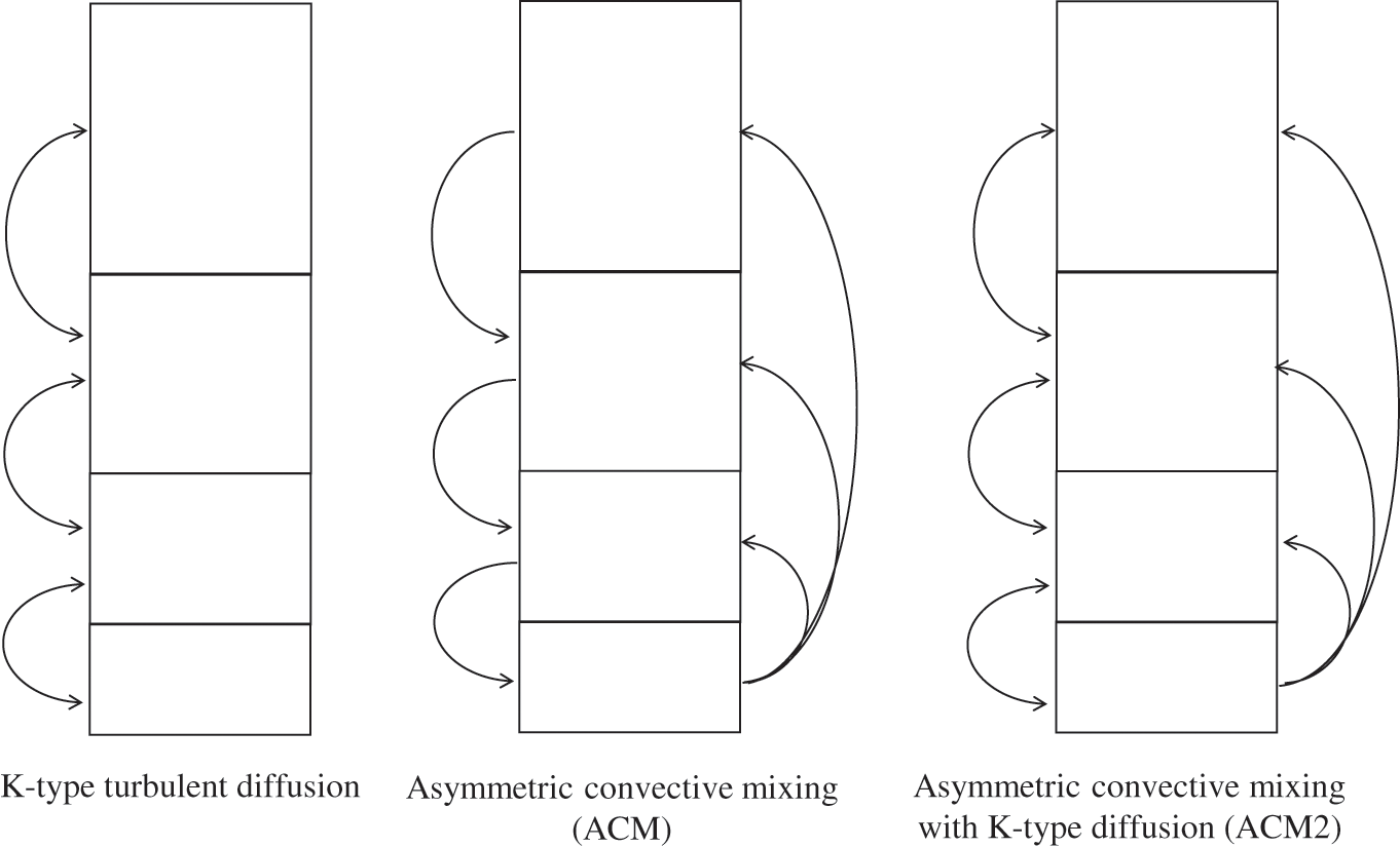
Figure 6.6. Schematic representations of vertical dispersion in eulerian models. Left figure: standard K-theory turbulent diffusion model; middle figure: convective dispersion model; right figure: model combining convective dispersion and K-theory turbulent diffusion.
The convective dispersion model presented here is the asymmetric convective mixing model (ACM). Mass transfer from the bottom layer occurs upward into all layers above. On the other hand, downward mass transfer occurs between adjacent layers (some earlier models used formulations allowing downward mass transfer among non-adjacent layers). The assumption used in ACM is that the upward mass transfer is due to strong convection, whereas downward transfer results from a slow subsidence and, therefore, is more gradual. Both approaches (K-theory and ACM) have been combined to provide a more complete representation of vertical mixing processes; the corresponding model is called ACM2 (Pleim, 2007).
Several parameterizations have been developed to represent the vertical turbulent diffusion coefficient, Kz, for models using K-theory for turbulence closure. For example, similarity theory may be used for the PBL to develop parameterizations of Kz (see Chapter 4). By analogy with the parameterization of the turbulent kinematic viscosity (i.e., the coefficient of turbulent transfer of momentum) presented in Equation 4.31, the following equation may be used for Kz:
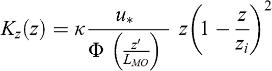 (6.59)
 where κ is the von Kármán constant (0.4), u* is the friction velocity (see Chapter 4.3), LMO is the Monin-Obukhov length, which characterizes atmospheric stability (see Chapter 4.4), z is altitude, zi is the PBL height, and z’ is equal to z, except for unstable conditions when z’ is the surface layer depth (0.1 zi) for z > z’. The PBL height, zi, is usually obtained from a meteorological numerical simulation; however, parameterizations are also available to estimate it (see for example, Troen and Mahrt, 1986). The function Φ varies depending on the atmospheric stability. Those presented in Equations 4.68 and 4.69 for heat transfer may be used for mass transfer. Figure 6.7 shows the vertical profile of this vertical dispersion coefficient for various atmospheric stability conditions.
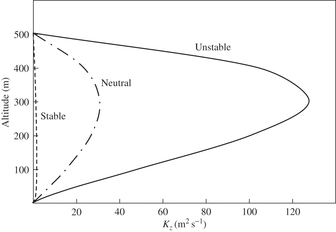
Figure 6.7. Vertical profiles of the eulerian vertical dispersion coefficient (similarity theory formulation). Meteorological conditions: stable (dashed line), neutral (dash-dotted line), and unstable (solid line). The PBL height is 500 m. The friction velocity (u*) is 0.3, 0.4, and 0.6 m s−1 for stable, neutral, and unstable conditions, respectively.
Other parameterizations of vertical dispersion have been developed for the PBL and the free troposphere. For example, the parameterization of Louis (1979) is used in many models for the PBL. Some other parameterizations use the convection velocity, rather than the friction velocity (e.g., Troen and Mart, 1986).
6.5.3 Horizontal Dispersion
Various formulations are available to parameterize the horizontal dispersion coefficient in eulerian chemical-transport models. These formulations depend usually on the horizontal grid size of the eulerian model. However, the dispersion coefficients depend on model grid size in ways that may lead to confusion: one formulation uses a proportional relationship between the dispersion coefficient and the grid surface area, whereas another formulation uses an inversely proportional relationship. The most widely used formulation is that of Smagorinsky (1963):
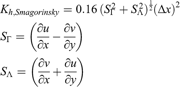 (6.60)
 where SΓ represents the stretching deformation and SΛ
 the shearing deformation of the wind field; Δx is the horizontal grid size (m). This formulation leads to a horizontal dispersion coefficient, which is proportional to the horizontal grid cell surface area. Therefore, horizontal dispersion will become very large for a model simulation where a large horizontal grid size is used (say >10 km). Since numerical diffusion increases with grid size, it is likely that the horizontal dispersion term will become superfluous when the horizontal model resolution is coarse. Thus, it appears that this formulation should be limited to cases where the model horizontal grid size, Δx, is on the order of a few km.
Another parameterization, called Unif, has been proposed to counter numerical diffusion in cases where a coarse horizontal resolution is used (Byun and Schere, 2006):
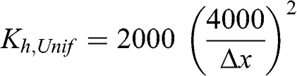 (6.61)
 This formulation leads to a horizontal dispersion coefficient, which is inversely proportional to the horizontal grid cell surface area, (Δx)−2. Therefore, its value decreases when Δx increases, i.e., when numerical diffusion increases. However, this formulation is not applicable to simulations where a very small grid size is used, because Kh tends toward infinity when the grid size decreases (for example, it is 32,000 m2 s−1 for Δx = 1 km).
An evaluation of these two formulations was performed using a field experiment conducted in 1999 in Texas. Tracer gases were released from different locations and measured downwind with a monitoring network. The model simulation used two imbedded domains with horizontal grid sizes of 12 and 4 km, respectively. The results suggested that, for this model configuration, the Smagorinsky formulation led to better model performance than the Unif formulation (Pun et al., 2006). Byun and Schere (2006) proposed the following formulation, which combines the two formulations previously described:
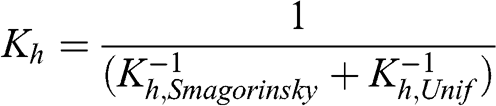 (6.62)
 When Δx tends toward 0, (Kh,Unif)−1 tends toward 0 and Kh tends toward Kh,Smagorinsky; when Δx tends toward infinity, (Kh,Smagorinsky)−1 tends toward 0 and Kh tends toward Kh,Unif. Figure 6.8 illustrates how these eulerian horizontal dispersion coefficients depend on the horizontal grid size.

Figure 6.8. Eulerian horizontal dispersion coefficients: Kh (solid line), Kh,Smagorinsky (dash-dotted line), Kh,Unif (dashed line). A value of 10−4 s−1 was used for the wind field deformation.
6.6 Street-canyon Models
The application of gaussian models to the urban canopy is strongly limited by the presence of buildings, which affect the air flow and, therefore, the transport and dispersion of air pollutants. In addition, the air pollution in a street canyon results mostly from local sources and it cannot be modeled by eulerian models, which have a grid resolution of at least 1 km, i.e., much greater than the dimension of a street canyon. Computational fluid dynamics (CFD) models can solve the equations that govern the air flow and the dispersion of the pollutants while taking into account the effect of buildings; however, the associated computational costs are too large to make CFD models applicable to large domains for long periods. Therefore, other approaches had to be developed to simulate the transport and dispersion of pollutants in an urban canopy with parameterizations that take into account the presence of buildings.
The most commonly used formulations are currently the Operational Street Pollution Model (OSPM; Berkowicz, 2000) and SIRANE (Soulhac et al., 2011). The latter is the most recent and it is summarized here. This formulation uses the assumption that the air pollutant concentration is uniform within a street canyon (or a segment of a street canyon). The turbulent transfer of air pollutants between the street canyon and the atmosphere above the urban canopy is modeled using a mass transfer coefficient at roof level. The horizontal transport of air pollutants within the street canyon is modeled using a wind that is parallel to the street axis, with a wind speed calculated using an exponential vertical profile. Then, the concentration of an air pollutant within the street canyon, C (g m−3), is calculated via a steady-state mass balance, which takes into account the pollutant emissions in the street as well as deposition processes:
 (6.63)
 where us is the mean wind speed within the street canyon (m s−1), σw is the standard deviation of the vertical wind speed at roof level (m s−1), hb, Ws, and Ls are the average height of the buildings, the average street width, and the length of the street-canyon segment, respectively (m), Sl is the emission rate of the pollutant in the street-canyon segment (g m−1 s−1), Cu is the concentration of the pollutant transported form the upwind street-canyon intersection (g m−3), Cb is the background concentration of the pollutant above the urban canopy (g m−3, concentration obtained either from air monitoring stations or from a model simulation), and Fd (g m−2 s−1) is the average dry deposition flux on urban surfaces (street, buildings … ). The average wind speed within the street is calculated using the assumption of an exponential vertical wind profile (see Equation 4.43) and accounting for the angle between the wind direction above the urban canopy and the direction of the street-canyon axis. The first term of the equation represents the pollutant inflow rate from the upwind intersection and the second term represents the emission rate within the street. The third term represents the outflow rate toward the downwind intersection. The fourth term represents dry deposition on surfaces. Scavenging by rain is not included here, but may easily be added if needed. The fifth term represents pollutant transfer between the street canyon and the background atmosphere above the urban canopy. It depends only on atmospheric turbulence (represented by σw) and does not account, for example, for traffic-generated turbulence or the effect of vegetation on atmospheric turbulence. Deposition fluxes may be calculated with parameterizations described in Chapter 11; they may be a function of surface type (street, sidewalk, building walls, windows, etc.).
SIRANE simulates the horizontal transport of air pollutants at street intersections by taking into account the variability of the wind direction and by conducting a mass balance of the flows through the intersection. Thus, some turbulent mass transfer at roof level is used to compensate for the horizontal inflows from and outflows to the street canyons connected with the intersection. The set of street-canyon equations is solved numerically, and the pollutant concentrations are calculated for each street-canyon segment.
If the wind is perpendicular to the street-canyon axis, an air recirculation zone may develop on the upwind side of the street while a ventilation zone may appear on the downwind side. Therefore, if an air pollutant is emitted within the recirculation zone, its concentration will be greater than that of an air pollutant emitted within the ventilation zone. The OSPM formulation takes into account the presence of recirculation and ventilation zones within a street-canyon configuration. However, the horizontal configuration of the street-canyon network may also generate recirculation zones and an academic representation of recirculation and ventilation zones may not always apply. Then, a CFD model is needed to simulate the air flow and calculate air pollutant concentrations in cases of complex configurations.
6.7 Numerical Modeling of Pollutant Transport in the Atmosphere
Gaussian plume models and street-canyon models have analytical solutions, which do not present any particular numerical difficulties. However, the calculation must be conducted for each source and receptor (i.e., the location where the air pollutant concentration is calculated) or for each street-canyon segment. Therefore, a large number of sources, receptors, and street-canyon segments may lead to significant computational costs.
Puff models require more computations, because puff trajectories must be tracked according to a wind field obtained from a numerical meteorological model. However, the computation of the pollutant concentrations within the puffs does not lead to any more numerical difficulties than those of gaussian plumes (puffs that treat chemical reactions may lead to numerical difficulties due to fast kinetics, see Chapter 7).
Eulerian chemical-transport models require a numerical solution of the set of the mass conservation equations representing the processes governing the concentrations of the air pollutants. Two distinct terms appear in the partial differential equation (excluding source, sink, and transformation terms): a term representing transport of the air pollutants by the mean wind and a turbulent dispersion term.
The first term (transport by the mean wind) is hyperbolic and presents a numerical difficulty: it leads to numerical diffusion, which artificially spreads concentrations throughout the model gridded system. Numerical diffusion may be reduced by using a finer spatial resolution, but, then, the computational cost increases considerably. Therefore, numerical algorithms have been developed to minimize numerical diffusion while keeping the computation costs manageable. However, some algorithms may have negative secondary effects such as the propagation of concentrations upwind (e.g., Bott’s algorithm) or non-conservation of mass (e.g., some semi-lagrangian algorithms based on spatial gradients). Decisions on the choice of a numerical algorithm must be made based on the application at hand. The Smolarkiewicz algorithm is widely used; it presents few shortcomings, however, it is more diffusive than some other algorithms. The piecewise parabolic method is used in several models, because it presents the advantage of being positive definite and monotonous (Colella and Woodward, 1984). The algorithm of Walcek and Aleksic (1998) is also monotonous and mass conserving; in addition, it may be used via operator splitting for both transport terms (mean wind transport and dispersion). Comparisons of numerical algorithms have been conducted, which provide valuable information on the pros and cons of various available algorithms (e.g., Dabdub and Seinfeld, 1994).
The second term (dispersion) is parabolic and, therefore, does not present any particular numerical difficulty. Standard numerical algorithms, such as semi-implicit methods, may be used (e.g., von Rosenberg, 1969).
Problems
Problem 6.1 Dispersion of a gaussian plume
A plume is emitted from an incinerator stack. Atmospheric conditions are assumed to be stationary, and a gaussian plume model is used to simulate the atmospheric dispersion of this plume. The dioxin emission rate is 6 × 10⁻⁴ g s−1, the stack height is 20 m, atmospheric stability is neutral, the wind speed is 5 m s−1, and plume rise is assumed to be negligible. Calculate the dioxin concentration, C, at a location 1 km downwind, underneath the plume at a height of 1.5 m corresponding to a person’s exposure.
Problem 6.2 Atmospheric dispersion of air pollutants
Air pollutants emitted from a tall stack lead to exceedance of an ambient air quality standard at a nearby monitoring station. Reducing the emissions with some control equipment would be too costly, and increasing the stack height is not allowed by the local regulatory agency. Suggest another approach to increase the dilution of the air pollutants in order to attain the ambient air quality standard.
Problem 6.3 Plume rise
Calculate the plume rise for a power plant stack with the following characteristics and atmospheric conditions: the stack diameter is 7.3 m, the plume initial vertical velocity at the stack exit is 18 m s−1, the plume initial temperature is 77 °C, the ambient temperature is 20 °C, and the horizontal wind speed is 5 m s−1.
Problem 6.4 Lagrangian and eulerian representations of atmospheric dispersion
The gaussian dispersion coefficients of McElroy-Pooler under rural conditions and neutral atmospheric stability are used here (Table 6.1) with a wind speed of 10 m s−1.
a. Calculate the corresponding eulerian coefficients.
b. At which downwind distance from the source can these eulerian dispersion coefficients be used?
c. Check whether the values of these eulerian dispersion coefficients are consistent with the values given in this chapter.