Abstract
Similar to the Archimedean copulas, the non-Archimedean copulas can be classified as one-parameter non-Archimedean bivariate copulas, two-parameter non-Archimedean bivariate copulas, and multivariate (d ≥ 3)d≥3) non-Archimedean copulas. In recent years, successful applications of non-Archimedean copulas, such as meta-elliptical copulas and Plackett copulas, have been reported in hydrology and water resources management. In this chapter, we will focus on Plackett copulas and more specifically bivariate and trivariate Plackett copula.
6.1 Bivariate Plackett Copula
In this section, we will introduce the definition, parameter estimation, as well as the random variate simulation with the use of bivariate Plackett copulas.
6.1.1 Definition of Bivariate Plackett Copula
As discussed in Chapter 3, the Plackett copula is constructed using the algebraic method. The cross-product ratio θθ, or odds ratio, is a measure of “association” or “dependence” in 2 × 22×2 contingency tables. Here, we label the categories for each variable as “low” and “high” and give four categories in Table 6.1, where a, b, c, and d represent the observed counts in the four categories, respectively. From Table 6.1, the cross-product ratio (θ : θ>0)θ:θ>0) is defined as θ=adbc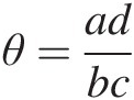 . Following Palaro and Hotta (2006), the dependence may be explained through θθ as follows:
1. 0 < θ < 10<θ<1 corresponds to negative dependence, i.e., observations are more concentrated in the “low-high” and “high-low” cells.
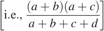
2. θ = 1θ=1 corresponds to independence, each “observed” entry; for example, a is equal to its “expected value” under independence [i.e.,a+ba+ca+b+c+d]
 .
.
3. θ>1θ>1 corresponds to positive dependence, i.e., observations are more concentrated in the “low-low” and “high-high” cells.
Table 6.1. Two-by-two contingency table.
| Column variable | ||||
|---|---|---|---|---|
| Row variable | Low (X ≤ xX≤x) | High (X>xX>x) | ||
| Low (Y ≤ y)Y≤y) | a | b | a+b | |
| High (Y>y)Y>y) | c | d | c+d | |
| a+c | b+d | a+b+c+d | ||
With the use of the 2 × 22×2 contingency table, Plackett (1965) developed what is now called the Plackett copula for bivariate continuous random variables. Assuming the continuous random variables X and Y with marginals FX and FYFXandFY and the joint distribution function H(x, y) = P(X ≤ x, Y ≤ y)Hxy=PX≤xY≤y, then the “low” and “high” categories for the column and row variables are replaced by events X ≤ x, X>xX≤x,X>x and Y ≤ y, Y>yY≤y,Y>y, respectively. According to the definition of cross-product ratio θ=adbc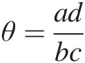 , it is clear that a, b, c, and d denote the probabilities of P(X ≤ x, Y ≤ y), P(X>x, Y ≤ y), P(X ≤ x, Y>y),PX≤xY≤y,PX>xY≤y,PX≤xY>y, and P(X>x, Y>y)PX>xY>y, respectively.
Now, based on the bivariate probability relation discussed in Chapter 3, we have the following:
Replacing the values of a, b, c, and d, we obtain the expression of parameter θ as follows:
 (6.1e)
Let u = FX(x)u=FXx and v = FY(y)v=FYy. Equation (6.1e) may be written in the copula form by applying Sklar’s theorem as follows:
 (6.2)
(6.2)Solving for C in Equation (6.2), we obtain the Plackett copula:
 (6.3a)
Taking the partial derivatives with respect to u and v, its copula density function can be written as follows:
 (6.4)
(6.4)Taking the partial derivative of equation (6.3a) with respect to u or v, the conditional probability distributions can be obtained as follows:
 (6.5)
(6.5) (6.6)
(6.6)Example 6.1 Graph the Plackett copula function and its density function with θ = 20, θ = 1, and θ = 0.5θ=20,θ=1,andθ=0.5.
Solution: Using Equations (6.3) and (6.4), we can graph the Plackett copula function and its density function in Figure 6.1 using u, v ∈ [0, 1]u,v∈01. From the copula density function plots with different parameters in Figure 6.1, it is seen that (i) the density is higher if both u and v take on smaller or bigger values at the same time for θ = 20θ=20, i.e., high follows high and low follows low as the representation of positive dependence; (ii) the density is constant, i.e., 1, if θ = 1θ=1 for the independent random variables; and (iii) the negative dependence is observed from the density function plot for θ = 0.5θ=0.5, in this case, smaller u and bigger v reach higher density and vice versa.

Figure 6.1 Plackett copula function and its density function plot for θ = 20, θ = 1 and θ = 0.5θ=20,θ=1andθ=0.5.
6.1.2 Simulation of Bivariate Plackett Copula
Following the Rosenblatt transform (Rosenblatt, 1952), the random variable can be simulated as follows:
1. Simulate two independent random variables (w1, w2)w1w2 from the uniform distribution U(0, 1)U01.
2. Set u = w1u=w1.
3. Using Equation (6.5a) and set w2 = C(v| u)w2=Cvu, i.e.,
w2=∂Cuvθ∂u=12+−1+u+v−uθ+vθ21+θ−1u+v2−4θθ−1uv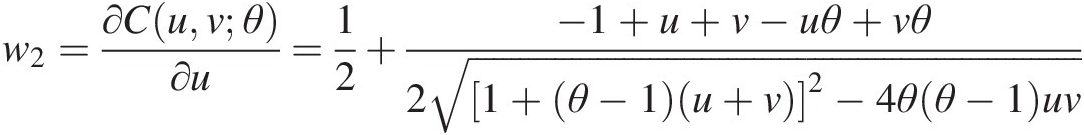 (6.7)
(6.7)

After some algebraic manipulation of Equation (6.7), vv can be solved as follows:
 (6.8)
(6.8)where
Example 6.2 Generate the random variables from the Plackett copula function.
To generate the variables, use the following information:
1. Simulate Plackett random variables from the uniformly distributed independent random variables w1 = 0.1645w1=0.1645, w2 = 0.9629w2=0.9629, and θ = 50θ=50.
2. Given θ = 50θ=50, θ = 2.5θ=2.5, and θ = 0.1θ=0.1, graph the the random variables generated from the Plackett copula with a sample size of 100.
Solution: We can use the procedure discussed in Section 6.1.2 to generate the random variables from Plackett copula:
1. w1 = 0.1645w1=0.1645, w2 = 0.9629w2=0.9629, and θ = 50θ=50.
Set u = w1 = 0.1645u=w1=0.1645. We may then compute the random variate vv using w2 = C(v| U = u; θ)w2=CvU=uθ.
Solving Equation (6.8), we have the following:
Then we have the following:
S = 0.0357; b = 135.7723; c = 75.8700; d = 69.6972S=0.0357;b=135.7723;c=75.8700;d=69.6972.
v=c−1−2w2d2b=75.8700−1−20.962969.69722135.7723=0.5170
Thus, the generated random variables are (u, v) = (0.1645, 0.5170)uv=0.16450.5170.
2. Set θ = 50θ=50, θ = 2.5θ=2.5 and θ = 0.1θ=0.1 with a sample size of 100.
Using the same procedure as in step 1, we graph the simulated random variables with a sample size of 100 in Figure 6.2. Again, Figure 6.2 clearly shows that (i) the random variables generated are positively dependent with θ = 50θ=50; (ii) the random variables generated are negatively dependent with θ = 0.1θ=0.1; and (iii) the random variables generated are more scattered within [0, 1]2 that are near independent when θ = 2.5θ=2.5.


Figure 6.2 Scatter plot of simulated random variables from the Plackett copula.
6.1.3 Parameter Estimation for Bivariate Plackett Copulas
As discussed in Section 3.6, the full ML, IFM, and semiparametric (pseudo-ML) methods may be applied to estimate the parameter numerically for the Plackett copula function. Here, without further discussion, we will give one example to illustrate the procedure of parameter estimation.
Example 6.3 Using the random variables (Table 6.2) and assuming (a) random variables X and Y are sampled from the normal distribution and gamma distribution, respectively, and (b) the joint distribution may be modeled using Plackett copula, estimate the parameters using full ML, IFM, and semiparametric methods.
Table 6.2. Sample data for Example 6.3.
| No. | X | Y | No. | X | Y |
|---|---|---|---|---|---|
| 1 | 11.276 | 5.049 | 26 | 12.793 | 12.942 |
| 2 | 19.570 | 12.015 | 27 | 16.772 | 4.140 |
| 3 | 10.864 | 3.691 | 28 | 12.215 | 4.522 |
| 4 | 14.517 | 9.233 | 29 | 24.909 | 7.689 |
| 5 | 17.512 | 6.862 | 30 | 17.580 | 12.331 |
| 6 | 14.312 | 5.343 | 31 | 17.200 | 7.060 |
| 7 | 17.785 | 12.689 | 32 | 10.621 | 5.583 |
| 8 | 9.457 | 8.182 | 33 | 10.310 | 19.026 |
| 9 | 13.290 | 8.531 | 34 | 8.957 | 3.648 |
| 10 | 15.470 | 31.129 | 35 | 18.735 | 7.534 |
| 11 | 18.392 | 20.848 | 36 | 11.536 | 7.519 |
| 12 | 9.411 | 8.567 | 37 | 16.264 | 10.727 |
| 13 | 18.883 | 15.874 | 38 | 21.382 | 21.947 |
| 14 | 11.749 | 12.142 | 39 | 19.153 | 11.813 |
| 15 | 14.173 | 10.224 | 40 | 17.355 | 7.988 |
| 16 | 14.044 | 6.223 | 41 | 17.877 | 12.159 |
| 17 | 13.032 | 7.594 | 42 | 14.799 | 9.622 |
| 18 | 18.374 | 14.827 | 43 | 11.457 | 11.147 |
| 19 | 17.979 | 14.283 | 44 | 18.601 | 14.626 |
| 20 | 7.656 | 4.639 | 45 | 11.636 | 4.732 |
| 21 | 14.642 | 10.039 | 46 | 11.427 | 6.263 |
| 22 | 19.871 | 16.856 | 47 | 15.067 | 11.378 |
| 23 | 7.769 | 17.575 | 48 | 16.328 | 14.778 |
| 24 | 12.870 | 7.763 | 49 | 21.471 | 29.678 |
| 25 | 14.119 | 6.964 | 50 | 15.327 | 9.639 |
Solution: With the assumption of X following the Gumbel distribution (Equation (2.10)) and Y following the gamma distribution (Equation (2.8)), applying MLE, we can initially estimate the parameters of random variables X and Y as follows:
Random variable X: μX = 14.9358; σX = 3.8484μX=14.9358;σX=3.8484.
Random variable Y: αY = 4.0031; βY = 0.3668αY=4.0031;βY=0.3668.
In addition, using Equation (3.72), we can compute the sample Kendall correlation coefficient as τn = 0.3690τn=0.3690.
1. Full ML Method:
As discussed in Section 3.6.1, we will need to estimate the parameters of marginal distributions and copula function simultaneously with the full log-likelihood function given as follows:
LL=∑ilncplackett(FXNormalxiμXσXFYGammayiαYβYθ+∑ilnfXNormalxiμXσX+∑ilnfYGammayiαYβY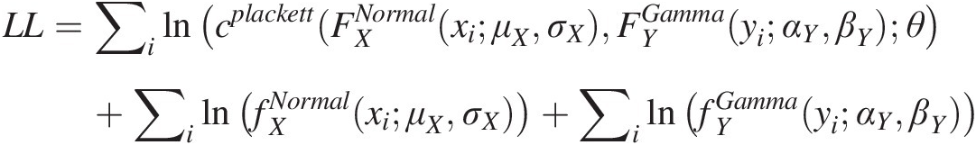
Using the parameters initially estimated for marginal distributions and assuming the initial estimate of the Plackett copula parameter θ = 10θ=10, we can use optimization toolbox in MATLAB to estimate the full set of parameters. The fitted marginal distribution is listed in Table 6.3 with the estimated parameters listed in Table 6.4.
2. IFM Method:
As discussed in Section 3.6.2, the parameters of marginal distributions and copulas are estimated separately with the use of IFM method. We will first compute the cumulative probability using the parameters initially estimated for the marginal distributions listed in Table 6.3. Then we will estimate the parameter of the Plackett copula using the ML method (the optimization toolbox in MATLAB) and the computed cumulative probabilities as random variates as follows:
LL=∑ilncplackettF̂Xxiμ̂Xσ̂XF̂Yyiα̂Yβ̂Yθ
The estimated copula parameter is listed in Table 6.4.
3. Semiparametric Method:
As discussed in Section 3.6.3, the semiparametric method is also called the pseudo-ML method. The marginal distributions are estimated nonparametrically using the Weibull plotting-position formula (Equation (3.92)) as listed in Table 6.3. Now with the use of the probability estimated nonparametrically, the pseudo-log-likelihood function can be written as follows:
LL=∑ilncplackettF̂nxiF̂nyiθ
The estimated parameter is again estimated using the optimization toolbox in MATLAB and listed in Table 6.4. From Table 6.4, it is seen that there is minimal difference in regard to the parameters of the marginal distributions estimated separately from the copula using the IFM method and those estimated simultaneously using the full ML method. Figure 6.3 further indicates this similarity through the univariate probability density comparison. Figure 6.4 compares the observed variates with the simulated variates from the fitted copula function. Figure 6.4 shows that the performances are very similar for the copulas with parameters estimated using three different techniques.


Table 6.3. Cumulative probability computed using the fitted normal and gamma distributions and Weibull probability plotting-position formula.
| X | FMLE | IFM | Empirical | Y | FMLE | IFM | Empirical |
|---|---|---|---|---|---|---|---|
| 19.570 | 0.871 | 0.882 | 0.900 | 12.015 | 0.638 | 0.633 | 0.640 |
| 10.864 | 0.129 | 0.141 | 0.160 | 3.691 | 0.047 | 0.045 | 0.040 |
| 14.517 | 0.427 | 0.449 | 0.460 | 9.233 | 0.434 | 0.428 | 0.460 |
| 17.512 | 0.724 | 0.742 | 0.680 | 6.862 | 0.242 | 0.237 | 0.220 |
| 14.312 | 0.406 | 0.428 | 0.440 | 5.343 | 0.132 | 0.129 | 0.140 |
| 17.785 | 0.747 | 0.764 | 0.720 | 12.689 | 0.680 | 0.675 | 0.720 |
| 9.457 | 0.067 | 0.075 | 0.100 | 8.182 | 0.348 | 0.343 | 0.400 |
| 13.290 | 0.308 | 0.328 | 0.360 | 8.531 | 0.377 | 0.371 | 0.420 |
| 15.470 | 0.526 | 0.548 | 0.560 | 31.129 | 0.996 | 0.996 | 0.980 |
| 18.392 | 0.795 | 0.810 | 0.800 | 20.848 | 0.946 | 0.944 | 0.920 |
| 9.411 | 0.065 | 0.073 | 0.080 | 8.567 | 0.380 | 0.374 | 0.440 |
| 18.883 | 0.829 | 0.843 | 0.860 | 15.874 | 0.830 | 0.827 | 0.840 |
| 11.749 | 0.183 | 0.199 | 0.260 | 12.142 | 0.646 | 0.641 | 0.660 |
| 14.173 | 0.392 | 0.414 | 0.420 | 10.224 | 0.512 | 0.506 | 0.540 |
| 14.044 | 0.380 | 0.401 | 0.380 | 6.223 | 0.193 | 0.189 | 0.180 |
| 13.032 | 0.284 | 0.304 | 0.340 | 7.594 | 0.300 | 0.295 | 0.320 |
| 18.374 | 0.794 | 0.809 | 0.780 | 14.827 | 0.789 | 0.785 | 0.820 |
| 17.979 | 0.763 | 0.780 | 0.760 | 14.283 | 0.764 | 0.760 | 0.760 |
| 7.656 | 0.025 | 0.028 | 0.020 | 4.639 | 0.091 | 0.088 | 0.100 |
| 14.642 | 0.440 | 0.462 | 0.480 | 10.039 | 0.498 | 0.492 | 0.520 |
| 19.871 | 0.887 | 0.897 | 0.920 | 16.856 | 0.863 | 0.860 | 0.860 |
| 7.769 | 0.026 | 0.030 | 0.040 | 17.575 | 0.883 | 0.881 | 0.880 |
| 12.870 | 0.270 | 0.289 | 0.320 | 7.763 | 0.314 | 0.309 | 0.360 |
| 14.119 | 0.387 | 0.409 | 0.400 | 6.964 | 0.250 | 0.245 | 0.240 |
| 12.793 | 0.264 | 0.282 | 0.300 | 12.942 | 0.694 | 0.690 | 0.740 |
| 16.772 | 0.656 | 0.676 | 0.620 | 4.140 | 0.066 | 0.064 | 0.060 |
| 12.215 | 0.217 | 0.234 | 0.280 | 4.522 | 0.085 | 0.082 | 0.080 |
| 24.909 | 0.994 | 0.995 | 0.980 | 7.689 | 0.308 | 0.303 | 0.340 |
| 17.580 | 0.730 | 0.748 | 0.700 | 12.331 | 0.658 | 0.653 | 0.700 |
| 17.200 | 0.696 | 0.715 | 0.640 | 7.060 | 0.257 | 0.253 | 0.260 |
| 10.621 | 0.116 | 0.127 | 0.140 | 5.583 | 0.148 | 0.145 | 0.160 |
| 10.310 | 0.101 | 0.111 | 0.120 | 19.026 | 0.916 | 0.914 | 0.900 |
| 8.957 | 0.052 | 0.058 | 0.060 | 3.648 | 0.045 | 0.044 | 0.020 |
| 18.735 | 0.819 | 0.833 | 0.840 | 7.534 | 0.295 | 0.290 | 0.300 |
| 11.536 | 0.169 | 0.184 | 0.220 | 7.519 | 0.294 | 0.289 | 0.280 |
| 16.264 | 0.607 | 0.628 | 0.580 | 10.727 | 0.549 | 0.544 | 0.560 |
| 21.382 | 0.945 | 0.951 | 0.940 | 21.947 | 0.959 | 0.958 | 0.940 |
| 19.153 | 0.847 | 0.859 | 0.880 | 11.813 | 0.625 | 0.620 | 0.620 |
| 17.355 | 0.710 | 0.729 | 0.660 | 7.988 | 0.332 | 0.327 | 0.380 |
| 17.877 | 0.755 | 0.772 | 0.740 | 12.159 | 0.647 | 0.642 | 0.680 |
| 14.799 | 0.456 | 0.478 | 0.500 | 9.622 | 0.465 | 0.459 | 0.480 |
| 11.457 | 0.164 | 0.178 | 0.200 | 11.147 | 0.579 | 0.574 | 0.580 |
| 18.601 | 0.810 | 0.824 | 0.820 | 14.626 | 0.780 | 0.776 | 0.780 |
| 11.636 | 0.175 | 0.191 | 0.240 | 4.732 | 0.096 | 0.093 | 0.120 |
| 11.427 | 0.162 | 0.176 | 0.180 | 6.263 | 0.196 | 0.192 | 0.200 |
| 15.067 | 0.484 | 0.506 | 0.520 | 11.378 | 0.596 | 0.590 | 0.600 |
| 16.328 | 0.613 | 0.634 | 0.600 | 14.778 | 0.787 | 0.783 | 0.800 |
| 21.471 | 0.948 | 0.953 | 0.960 | 29.678 | 0.995 | 0.994 | 0.960 |
| 15.327 | 0.511 | 0.533 | 0.540 | 9.639 | 0.466 | 0.461 | 0.500 |
Table 6.4. Estimated parameters using the preceding three methods.
| Method | Univariate | Copula | ||
|---|---|---|---|---|
| X~normal | Y~Gamma | θθ | LL | |
| Full ML | (15.224, 3.846) | (4.039, 0.369) | 7.500 | –275.327 |
| IFM | (15.011, 3.851) | (4.069, 0.369) | 7.167 | 8.106 |
| Semiparametric | — | — | 7.759 | 8.464 |

Figure 6.3 Comparison of frequency and the fitted probability distributions using IFM and Full MLE.

Figure 6.4 Comparison of observations with simulated random variables with three estimation methods.
Example 6.4 Using the sample data and the parameters estimated with the IFM method in Example 6.3, compute the joint return period and conditional return period of
Solution: Applying the parameters estimated for the marginal distributions listed in Table 6.4 for the IFM method, we have
i. T(X>19 ∩ Y>21)TX>19∩Y>21
In this case, we are evaluating the recurrence interval if both X and Y exceed the value given in the preceding. Applying Equation (3.127) for the “and” case, we have the following:
F(X>19 ∩ Y>21)=1−FX(X≤19)−FY(Y≤21)+F(X≤19,Y≤21)=1−FX(X≤19)−FY(Y≤21)+Cplackett(FX(X≤19),FY(Y≤21);θ)=1−0.850−0.946+Cplackett(0.850,0.946;7.167)=1−0.850−0.946+0.824=0.028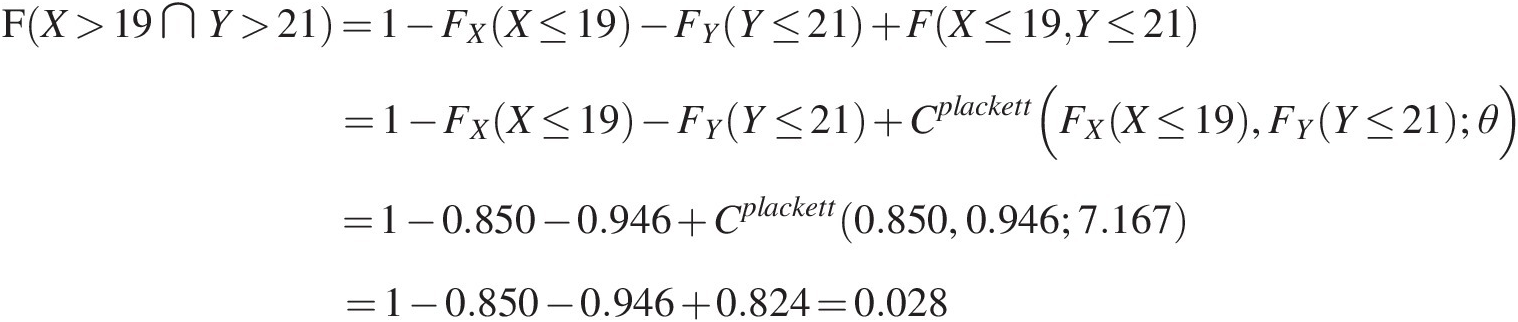
TX>19∩Y>21=1FX>19∩Y>21=10.028=36.10time units
ii. T(X>19| Y>21)TX>19Y>21
In this case, we are evaluating the recurrence interval of X > 19 under the condition of Y > 21:
F(X>19|Y>21)=F(X>19∩Y>21)F(Y>21)=1−FX(X≤19)−FY(Y≤21)+Cplackett(FX(X≤19),FY(Y≤21);θ)1−F(Y≤21)=1−0.850−0.946+0.8241−0.946=0.0280.054=0.516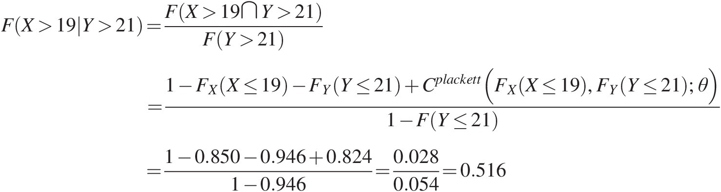
Applying Equation (2.91), we have the following:
TX>19Y>21=11−FYy≤2111−FXx≤19−FYY≤21+CplackettFXFYθ=10.053710.0277≈672time units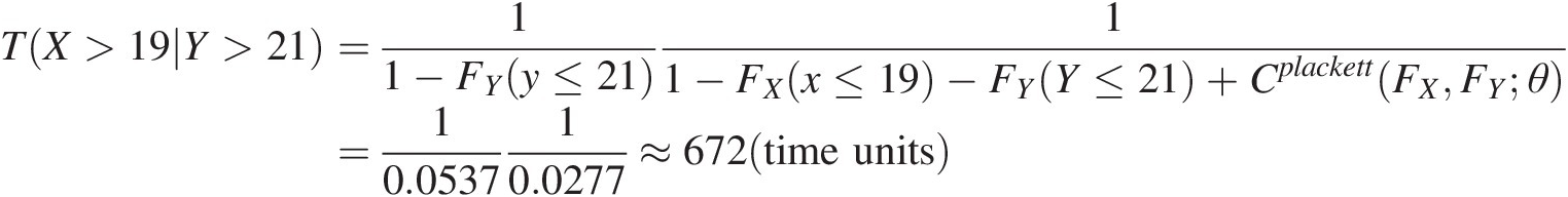
iii. T(X>19| Y = 21)TX>19Y=21


In this case, we are evaluating the recurrence interval of X > 19 under the condition that Y is exactly equal to 21:

Comparing the joint return period with the two conditional return periods we calculated, it is seen that the recurrence interval is longest for the conditional return period of (X>19| Y>21).X>19Y>21.
6.2 Trivariate Plackett Copula
In this section, we will focus on the trivariate Plackett copula, including its definition, the derivation of trivariate Plackett copula density, and a brief introduction of the parameter estimation method. Given the complexity of parameter estimation for the trivariate Plackett copula and the simplicity of other multivariate copula approaches, we will not further discuss the simulation as well as the formal goodness-of-fit measure in detail.
6.2.1 Definition of Cross-Product Ratio for the Trivariate Plackett Copula
For the given (u, v, wu,v,w), there are three compatible bivariate copulas: CUV, CVWCUV,CVW, and CUWCUW. Analogous to the bivariate case, the trivariate constant cross-product ratio θUVWθUVW can be defined following Kao and Govindaraju (2008), Song and Singh (2010) as
 (6.9)
(6.9)where
 (6.10)
Here CUV, CVWCUV,CVW, and CUWCUW are bivariate Plackett copulas with dependence parameters θUV, θVWθUV,θVW, and θUWθUW, for the given θUVWθUVW. Denoting z = CUVW(u, v, w)z=CUVWuvw, one can compute CUVW(u, v, w)CUVWuvw as follows:
where
 (6.12)
For the given θUV, θVW, θUWθUV,θVW,θUW, and θUVWθUVW, the corresponding trivariate Plackett copula may be obtained from Equations (6.11) and (6.12). For CUVW(u, v, w)CUVWuvw to be a valid three-copula, the following conditions needs to be satisfied:
1. Since each component in Equation (6.11) is a probability measure, we have the following:
CUVW(u, v, w) ∈ [b, a], b = max (0, b1, b2, b3); a = min (a1, a2, a3, a4)CUVWuvw∈ba,b=max0b1b2b3;a=mina1a2a3a4(6.13)
2. Equation (6.13) is the Fréchet–Hoeffding bounds for trivairate joint distributions with the known bivariate joint distributions (Joe, 1997).
3. As discussed in Section 3.1.2 of Chapter 3, Equations (3.23)–(3.26) need to be satisfied.
4. The copula density is CUVWuvw=∂3CUVWuvw∂u∂v∂w≥0
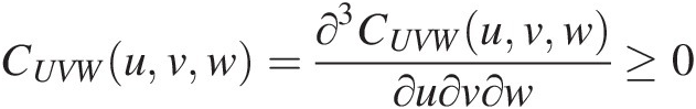 . Following Kao and Govidaraju (2008), the derivation of the density function will be discussed in Section 6.2.2.

With the fulfillment of the preceding four conditions, for the given cross-product ratio parameters θUV, θVW, θUWθUV,θVW,θUW, and θUVWθUVW, z = CUVW(u, v, w)z=CUVWuvw may be computed numerically with the following steps:
1. Compute CUV, CVW, and CUW using Equation (6.3).
2. To compute CUVWCUVW, Equation (5.11) can be rewritten as follows:
θUVW−1z4+−θUVWa1+a2+a3+a4+(b1+b2+b3]2+θUVWa1a2+a1+a2a3+a4+a3a4−b1b2+b3b1+b2z2+−θUVWa1a2a3+a4+a3a4a1+a2+b1b2b3z+θUVWa1a2a3a4=0Let f(z) represent the left side of Equation (6.14). We may use Newton’s iterative method to compute z numerically as follows: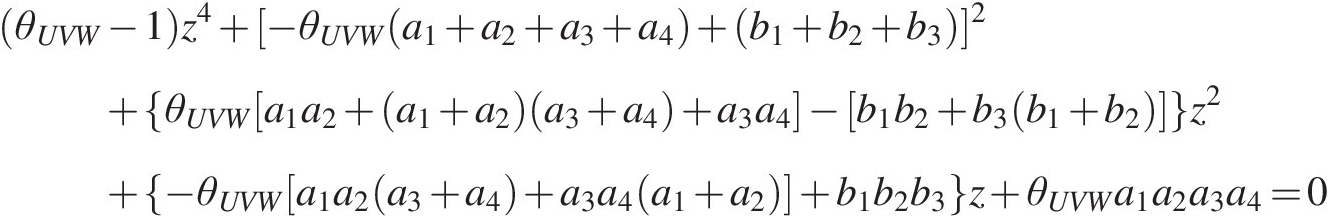 (6.14)
zn+1=zn−fznf’znwhere f‘(z)f′z is the first derivative of f(z)fz with respect to z; znzn and zn + 1zn+1 are the nth and (n+1)th iteratively computed values of z.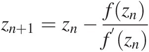 (6.15)


6.2.2 Derivation of Density Function of the Trivariate Plackett Copula
Following Kao and Govindaraju (2008), the density function of trivariate Plackett copula may be derived in the following manner:
1. Solve CUVWCUVW using given parameter θUVWθUVW and known bivariate copulas from Equation (6.11) or equivalently Equation (6.14).
2. Compute first-order derivatives of ∂CUV∂u,∂CUV∂v,∂CUW∂u,∂CUW∂w,∂CVW∂v
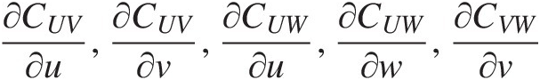 , and ∂CVW∂w
 from the corresponding known bivariate copulas. Similar to the vine copula discussed in Chapter 4, these bivariate copulas are not required to belong to the Plackett copula family, and each may belong to a different copula family.
3. Compute the first-order derivatives of P000, P010, P100, P011, P110, P101, P011P000,P010,P100,P011,P110,P101,P011, and P111P111 with respect to u, v, w, respectively, as follows:
∂P000∂u=−∂P100∂u=∂CUVW∂u∂P010∂u=−∂P110∂u=−∂CUVW∂u+∂CUW∂u∂P001∂u=−∂P101∂u=−∂CUVW∂u+∂CUV∂u∂P011∂u=−∂P111∂u=∂CUVW∂u−∂CUV∂u−∂CUW∂u+1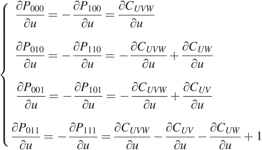 (6.16)
∂P000∂v=−∂P010∂v=∂CUVW∂v∂P100∂v=−∂P110∂v=−∂CUVW∂v+∂CVW∂v∂P001∂v=−∂P011∂v=−∂CUVW∂v+∂CUV∂v∂P101∂v=−∂P111∂v=∂CUVW∂v−∂CUV∂v−∂CVW∂v+1 (6.17)
∂P000∂w=−∂P001∂w=∂CUVW∂w∂P100∂w=−∂P101∂w=−∂CUVW∂w+∂CVW∂w∂P010∂w=−∂P011∂w=−∂CUVW∂w+∂CUW∂w∂P110∂w=−∂P111∂w=∂CUVW∂w−∂CUW∂w−∂CVW∂w+1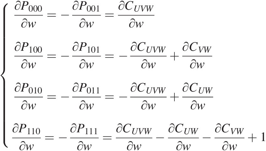 (6.18)
4. Compute ∂CUVW∂u,∂CUVW∂v,∂CUVW∂w
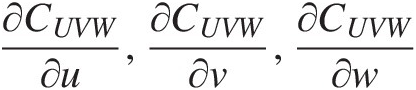 as follows:
∂P000∂uP011P101P110+P000∂P011∂uP101P110+P000P011∂P101∂uP110+P000P011P101∂P110∂u–θUVW(∂P111∂uP100P010P001+P111∂P100∂uP010P001+P111P100∂P010∂uP001+P111P110P101∂P110∂u)=0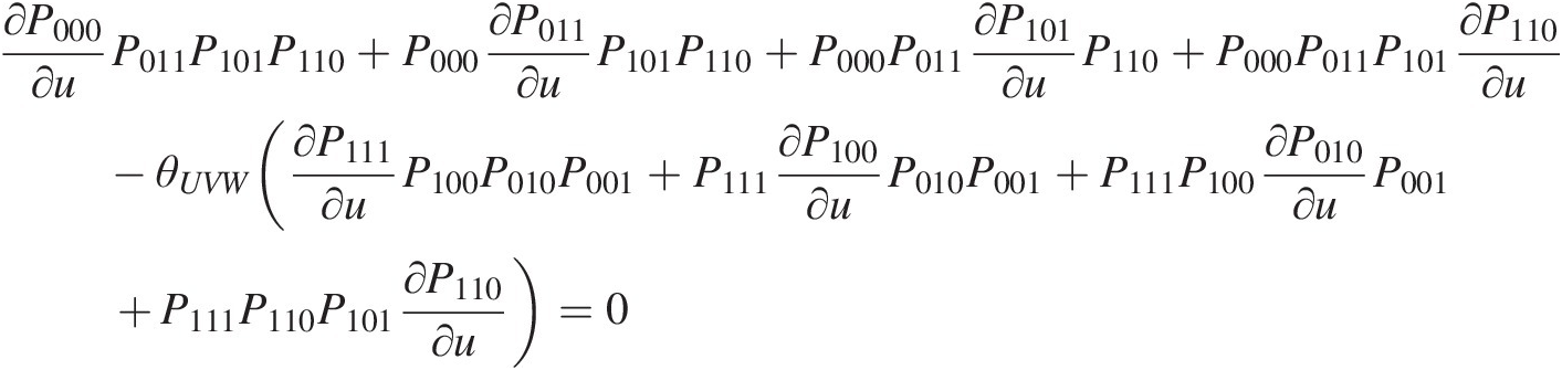 (6.19)
∂P000∂vP011P101P110+P000∂P011∂vP101P110+P000P011∂P101∂vP110+P000P011P101∂P110∂v–θUVW(∂P111∂vP100P010P001+P111∂P100∂vP010P001+P111P100∂P010∂vP001+P111P110P101∂P110∂v)=0 (6.20)
∂P000∂wP011P101P110+P000∂P011∂wP101P110+P000P011∂P101∂wP110+P000P011P101∂P110∂w–θUVW(∂P111∂wP100P010P001+P111∂P100∂wP010P001+P111P100∂P010∂wP001+P111P110P101∂P110∂w)=0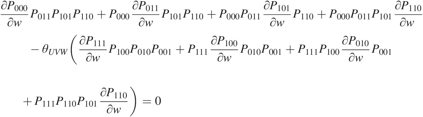 (6.21)
5. Compute the bivariate density function of cUV, cVW, cUWcUV,cVW,cUW.
6. Compute the second-order derivative of P000, P010, P100, P011, P110, P101, P011P000,P010,P100,P011,P110,P101,P011, and P111P111 with respect to u, v, w, respectively, as follows:
∂2P000∂u∂v=−∂2P100∂u∂v=−∂2P010∂u∂v=∂2P110∂u∂v=∂2CUVW∂u∂v∂2P001∂u∂v=−∂2P101∂u∂v=−∂2P011∂u∂v=∂2P111∂u∂v=−∂2CUVW∂u∂v+∂2CUV∂u∂v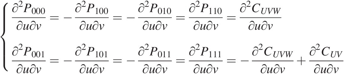 (6.22)
∂2P000∂u∂w=−∂2P100∂u∂w=−∂2P001∂u∂w=∂2P101∂u∂w=∂2CUVW∂u∂w∂2P010∂u∂w=−∂2P110∂u∂w=−∂2P011∂u∂w=∂2P111∂u∂v=−∂2CUVW∂u∂w+∂2CUW∂u∂w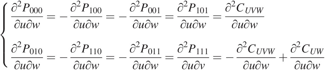 (6.23)
∂2P000∂v∂w=−∂2P010∂v∂w=−∂2P001∂v∂w=∂2P011∂v∂w=∂2CUVW∂v∂w∂2P100∂v∂w=−∂2P110∂v∂w=−∂2P101∂v∂w=∂2P111∂v∂w=−∂2CUVW∂v∂w+∂2CVW∂v∂w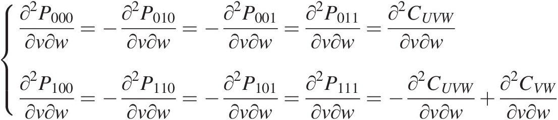 (6.24)
7. Compute ∂2CUVW∂u∂v,∂2CUVW∂v∂w,∂2CUVW∂u∂w
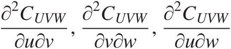 . As an example, ∂2CUVW∂u∂v
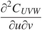 may be computed by applying ∂∂v
 to Equation (6.19) as follows:
∂2P000∂u∂vP011P101P110+∂P000∂u∂P011∂vP101P110+∂P000∂uP011∂P101∂vP110+∂P000∂vP011P101∂P110∂v+∂P000∂v∂P011∂uP101P110+P000∂2P011∂u∂vP101P110+P000∂P011∂u∂P101∂vP110+P000∂P011∂uP101∂P110∂v+∂P000∂vP011∂P101∂uP110+P000∂P011∂v∂P101∂uP110+P000P011∂2P101∂u∂vP110+P000P011P101∂u∂P110∂v+∂P000∂vP011P101∂P110∂u+P000∂P011∂vP101∂P110∂u+P000P011∂P101∂v∂P110∂u+P000P011P101∂2P110∂u∂v−θUVW(∂2P111∂u∂vP100P010P001+∂P111∂u∂P100∂vP010P001+∂P111∂uP100∂P010∂vP001+∂P111∂uP100P010∂P001∂v+∂P111∂v∂P100∂uP010P001+P111∂2P100∂u∂vP010P001+P111∂P100∂u∂P010∂vP001+P111∂P100∂uP010∂P001∂v+∂P111∂vP100∂P010∂uP001+P111∂P100∂v∂P010∂uP001+P111P100∂2P010∂u∂vP001+P111P100∂P010∂u∂P001∂v+∂P111∂vP100P010∂P001∂u+P111∂P100∂vP010∂P001∂u+P111P100∂P010∂v∂P001∂u+P111P100P010∂2P001∂u∂v)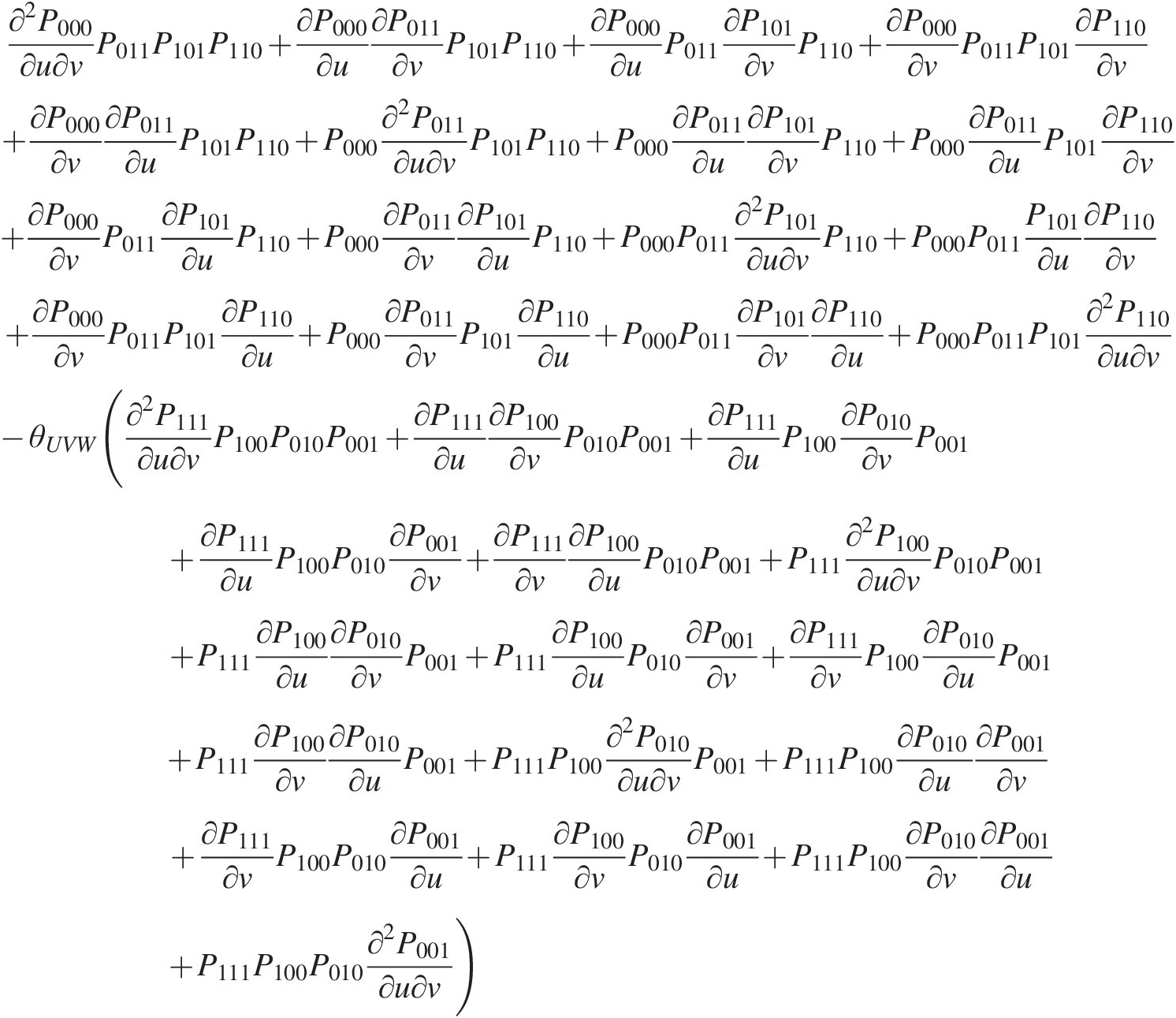 (6.25)
Similarly, applying ∂∂w,∂∂u
 , we can obtain ∂2CUVW∂v∂w,∂2CUVW∂u∂w
 from Equations (6.20) and (6.21), respectively.
8. Compute the probability density function ∂3CUVW∂u∂v∂w
 for the trivariate Plackett copula.
Applying ∂∂w
 to Equation (6.22), we have the following:
∂3P000∂u∂v∂w=−∂3P100∂u∂v∂w=−∂3P010∂u∂v∂w=∂3P110∂u∂v∂w=∂3CUVW∂u∂v∂w∂3P001∂u∂v∂w=−∂3P101∂u∂v∂w=−∂3P011∂u∂v∂w=∂3P111∂u∂v∂w=−∂3CUVW∂u∂v∂w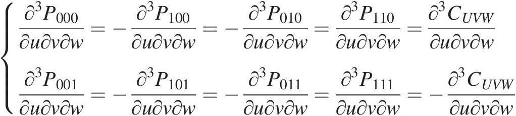 (6.26)
Applying ∂∂w
 to Equation (6.25), we obtain a new third-order derivative equation (we omit the derivative here). Substituting Equation (6.26) into the new equation derived for the third-order derivative, we have the density function as a function of P000, P011, P101, P110, P111, P010, P010, P001P000,P011,P101,P110,P111,P010,P010,P001.


Example 6.5 Express the PDF of trivariate Plackette copula with the following information:θUVW = 20; θUV = 15; θUW = 1.3; θVW = 1.4; u = 0.5; v = 0.975; w = 0.975θUVW=20;θUV=15;θUW=1.3;θVW=1.4;u=0.5;v=0.975;w=0.975
Solution: Applying the equations derived for the trivariate Plackett copula, we can compute the trivariate Plackett copula density function by following these procedure and steps:
1. Compute the bivariate Plackett copula for the paired variables with Equation (6.3); using bivariate variable (u, v)uv as an example, we have the following:
a3=CUV=CUV(0.5,0.975;15) =[1+(15−1)(0.5+0.975)]−[1+(15−1)(0.5+0.975)]2−4(15)(15−1)(0.5)(0.975)2(15−1)=0.498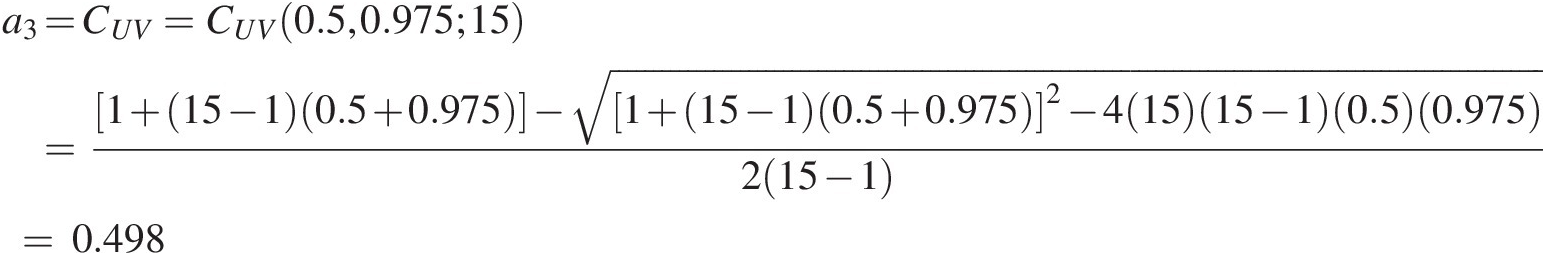
Similarly, we have the following:
a2 = CUW = CUW(0.5, 0.975; 1.3) = 0.489a2=CUW=CUW0.50.9751.3=0.489
a1 = CVW = CVW(0.975, 0.975; 1.4) = 0.951a1=CVW=CVW0.9750.9751.4=0.951
2. Compute the trivariate Plackett copula value using Equation (6.14), and solve it numerically as follows: CUVW(0.5, 0.975, 0.975; [15, 1.4, 1.3, 20]) = 0.488CUVW0.50.9750.975151.41.320=0.488
where the remaining a‘sa′s and b‘sb′s needed in Equation (6.12) are computed as follows:
a4 = 1 − 0.5 − 0.975 − 0.975 + 0.498 + 0.589 + 0.951 = 0.488a4=1−0.5−0.975−0.975+0.498+0.589+0.951=0.488
b1 = 0.489 + 0.951 − 0.975 = 0.465b1=0.489+0.951−0.975=0.465
b2 = 0.498 + 0.951 − 0.975 = 0.474b2=0.498+0.951−0.975=0.474
b3 = 0.498 + 0.489 − 0.5 = 0.487b3=0.498+0.489−0.5=0.487
3. Compute the derivatives needed to compute the trivariate Plackett density:
P000 = CUVW = 0.488, P100 = CVW − CUVW = 0.463,P000=CUVW=0.488,P100=CVW−CUVW=0.463,
P010 = CUW − CUVW = 7.903 × 10⁻⁴, P001 = CUV − CUVW = 0.0074,P010=CUW−CUVW=7.903×10⁻⁴,P001=CUV−CUVW=0.0074,
P110 = w − CUW − CVW + CUVW = − 0.0234, P101 = v − CUV − CVW + CUVW = 0.017P110=w−CUW−CVW+CUVW=−0.0234,P101=v−CUV−CVW+CUVW=0.017
P011 = u − CUV − CUW + CUVW = 0.004P011=u−CUV−CUW+CUVW=0.004
P111 = 1 − u − v − w + CUV + CVW + CUW − CUVW = − 0.003P111=1−u−v−w+CUV+CVW+CUW−CUVW=−0.003
The rest computation will need to apply the numerical method (i.e., Newton’s method). Here we will only lists the final results:
∂2CUV∂u∂v=0.594;∂2CUW∂u∂w=0.985;∂2CVW∂v∂w=1.348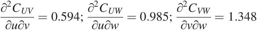
∂P000∂u=0.015;∂P111∂v=0.697;∂P111∂w=1.9461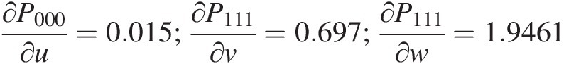
∂CUVW∂u=0.946;∂CUVW∂v=−0.555;∂CUVW∂w=1.542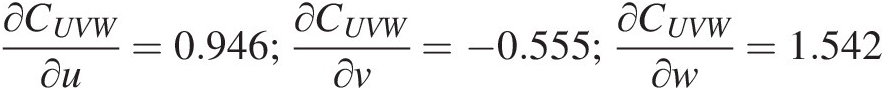
∂2CUVW∂u∂v=9.101;∂2CUVW∂u∂w=29.094;∂2CUVW∂v∂w=458.057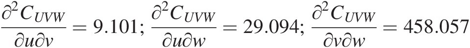


Finally, we have the trivariate Plackett copula density as follows:

6.2.3 Estimation of Cross-Product Ratio (Copula Parameter) for the Trivariate Plackett Copula
Following the same procedure for the bivariate Plackett copula, the parameter for the trivariate Plackett copula may be estimated. For a trivariate sample of X = {xi1, xi2, xi3, i = 1, …n}X=xi1xi2xi3i=1…n with ui1 = F1(xi1), ui2 = F2(xi2), ui3 = F3(xi3),ui1=F1xi1,ui2=F2xi2,ui3=F3xi3, we can then write the pseudo-MLE as follows:
 (6.27)
Taking the derivative with respect to θUVWθUVW and setting the derivative equal to 0, we have the following:
 (6.27a)
As shown in the previous section, the trivariate Plackett copula does not have an analytical form of the trivariate Plackett copula density function, and the parameter may be optimized by the numerical scheme (e.g., central differencing). Compared to the bivariate case, the parameter estimation of the trivariate Plackett copula is more tedious. It holds true, compared to the asymmetric Archimedean, vine, and meta-elliptical copulas.
6.3 Summary
In this chapter, we introduce the bivariate and trivariate Plackett copulas with the focus on the bivariate Plackett copula. The parameter estimation for the trivariate Plackett copulas is rather complex, compared to the trivariate asymmetric Archimedean, vine, and meta-elliptical copulas. Additionally, there does not exist the analytical form for the trivariate Plackett copula density. In general, it is recommended to apply asymmetric Archimedean, vine, and meta-elliptical copulas to model the multivariate dimensional dependence.