Abstract
Meta-elliptical copulas are derived from elliptical distributions. Kotz and Nadarajah (2001) and Nadarajah (2006) made solutions of meta-elliptical copulas available. In this chapter, we will review the definition and probability distributions as well as other properties of meta-elliptical copulas.
7.1 Meta-Elliptical Copulas
7.1.1 d-Dimensional Symmetric Elliptical Type Distribution
In previous chapters, we have discussed symmetric and asymmetric (i.e., nested) Archimedean copulas for multivariate modeling (i.e., d ≥ 3d≥3). We have shown that (i) symmetric multivariate Archimedean copulas require that all the correlated variables share the same dependence structure, and (ii) the nested asymmetric multivariate copulas still require that some variables share the same dependence structure. Compared to the symmetric and nested asymmetric Archimedean copulas, the meta-elliptical copulas are more flexible than the symmetric (or nested) Archimedean copulas for modeling multivariate hydrological variables.
Following Genest et al. (2007), a d-dimensional random vector z (z = [z1, …, zd]Tz=z1…zdT) is said to have an elliptical joint distribution, i.e., ℰd(μ, Σ, g)ℰdμΣg with mean vector μ(d × 1)μd×1, covariance matrix Σ(d × d)Σd×d, and generator g : [0, ∞)→[0, ∞)g:0∞→0∞, if there exists a stochastic representation, as follows:
where r ≥ 0r≥0 is a random variable with the probability density function as
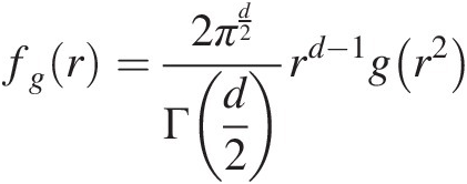 (7.1a)
u (independent of r) is uniformly distributed on the sphere as follows:
 (7.1b)
A is Cholesky decomposition of Σ, i.e., AAT = ΣAAT=Σ
and the joint probability density function of z can be written as follows:
 (7.2)
(7.2)In Equations (7.1a) and (7.2), g(⋅)g⋅ is a scale function uniquely determined by the distribution of r and referred to as the probability density function generator. Common d-dimensional symmetric elliptical type distribution generators are given in Table 7.1.
Table 7.1. Common probability density function generators [g(t)gt] for elliptical copulas.
| Copula | g(t)gt |
|---|---|
| Normal | 2π−d2exp−t2 |
| Student | πv−d2Γd+v2Γd21+tv−d+v2 |
| Cauchy | π−d2Γd+12Γ121+t−d+12 |
| Kotza | sΓd2r2N+d−22stN−1exp−rtsπd2Γ2N+d−22s;r,s>0,2N+d>2 |
| Pearson type II | Γd2+m+1πd2Γm+11−tm;t∈−11,m>−1 |
| Pearson type VIIb | ΓNΓN−d2πmd21+tm−N;N>d2,m>0 |
Notes:
a Kotz type copula reduces to normal copula if N = s = 1, r = 1/2N=s=1,r=1/2.
b Pearson type VII copula reduces to Cauchy copula if m = 1, N = 3/2m=1,N=3/2 and reduces to Student copula if N=m2+1 .
.
To build the meta-elliptical copula using the g(⋅)g⋅ function (listed in Table 7.1) and Equation (7.2), we should note that there is one limitation of these elliptical distributions, that is, the scaled variables z1σ11,z2σ22,…,zdσdd are identically distributed with the density function as follows:
 (7.3)
(7.3)and the CDF of the scaled variables given as follows:
 (7.4)
(7.4)From Equations (7.3) and (7.4), it is known that qg(x) = qg(−x)qgx=qg−x and Qg(x) = 1 − Qg(x) forx>0Qgx=1−Qgxforx>0.
Example 7.1 Derive the d-dimensional multivariate normal density function: z = [z1, …, zd]z=z1…zd.
Solution: As listed in Table 7.1, the probability density function generator for the multivariate normal distribution is gt=2π−d2exp−t2 . Applying Equation (7.2), we have the following:
 (7.5)
(7.5)If μ = 0μ=0 in Equation (7.5), we have
 (7.6a)
By applying Equation (7.1), we have zTΣ−1z = r2(Au)TΣ−1(Au) = r2zTΣ−1z=r2AuTΣ−1Au=r2 and Equation (7.6a) may be rewritten as follows:
 (7.6b)
where
Σ=ρ11⋯ρ1d⋮⋱⋮ρd1⋯ρdd,ρii=1;∣ρij∣<1,i≠j;i,j=1,..,d , correlation matrix.
Example 7.2 Derive the d-dimensional multivariate Cauchy density function for z = [z1, …, zd]z=z1…zd.
Solution: Using the probability density function generator for the multivariate Cauchy distribution listed in Table 7.1:

Applying Equation (7.2), we have the following:
 (7.7)
(7.7)Similarly, if μ = 0μ=0, we have from Equation (7.7) the following:
 (7.7a)
Or equivalently
 (7.7b)
Without loss of generality, we will only investigate the case ℰd(0, Σ, g)ℰd0Σg. Let z = [z1, z2, …, zd]Tz=z1z2…zdT be a random vector with each component zizi with given continuous PDF fi(zi)fizi and CDF Fi(zi)Fizi. Suppose
 (7.8)
(7.8)where Qg−1 is the inverse of QgQg.
Then, the probability density function of z is given by
where the Jacobian matrix J is given as follows:

Since xi=Qg−1Fizi , we have ∂xi∂zj=dxidzi,i=j0,i≠j
 . Rewriting matrix J, we have the following:

From xi=Qg−1Fizi , we have Fi(zi) = Qg(xi)Fizi=Qgxi. Differentiation on both sides leads to fi(zi)dzi = qg(xi)dxifizidzi=qgxidxi; dxidzi=fiziqgxi=fiziqg(Qg−1Fizi⇒J=∏i=1dfiziqgQg−1Fizi
Then, we have the following:
 (7.10)
For x = (x1, …, xd)T~ℰd(0, Σ, g)x=x1…xdT~ℰd0Σg, we have the following:
 (7.11)
Inserting Equation (7.11) in Equation (7.10), we have the following:
 (7.12)
Using ℋℋ to represent the d-variant probability density function as

Equation (7.12) may be written as follows:
 (7.12a)
To this end, the d-dimensional random vector z is said to have a meta-elliptical distribution, if its probability density function is given by Equation (7.12). Denote x~ℳℰd(0, Σ, g; F1, …, Fd)x~ℳℰd0ΣgF1…Fd. The function ℋQg−1F1z1…Qg−1Fdzd is referred to as the probability density function weighting function. The class of meta-elliptical distributions includes various distributions, such as elliptically contoured distributions, the meta-Gaussian distributions, and various asymmetric distributions. The marginal distributions Fi.
 can be arbitrarily chosen (Fang et al., 2002). The meta-elliptical distributions allow for the possibility of capturing tail dependence (Joe, 1997), which will be discussed later.
7.1.2 Bivariate Symmetric Elliptical Type Distribution
Suppose x~ℳℰ2(0, Σ, g)x~ℳℰ20Σg, we have the following:


Vector x has the following probability density function:
 (7.13)
The marginal PDF and CDF of x are
 (7.14)
 (7.15)
A two-dimensional random vector (x1, x2)x1x2 follows an elliptically contoured distribution, if its joint PDF takes on the form of Equation (7.13). Its copula function can be written as follows:
 (7.16)
where u=F1x1,v=F2x2,s=Qg−1u,t=Qg−1v .
.
The copula density function can be given as follows:
where
 (7.18)
Now, let z = (z1, z2)T~ℳℰ2(0, Σ, g; F1, F2)z=z1z2T~ℳℰ20ΣgF1F2. Its probability density function may then be expressed as follows:
 (7.19)
Take simple examples to illustrate the preceding.
Symmetric Kotz Type Distribution
Let x be distributed according to a bivariate symmetric Kotz type distribution. Inserting the density generator for Kotz type distribution (listed in Table 7.1) in Equation (7.2), we obtain the joint probability density function as follows:
 (7.20)
where r>0, s>0, N>0r>0,s>0,N>0 are the parameters.
The marginal PDF (i.e., q1(x)q1x) can be written as follows:
 (7.21)
The corresponding CDF (i.e., Q1(x)Q1x) can be written as follows:
 (7.22)
Then, the copula probability density function can be given as follows:
 (7.23)
Example 7.3 Show that the bivariate Kotz type distribution converges to the bivariate Gaussian distribution as noted in Table 7.1, i.e., N = s = 1, r = 1/2N=s=1,r=1/2.
Solution: Substituting N=s=1,r=12 into the probability density function generator of symmetric Kotz type distribution, we have

Comparing with the probability density function generator for the normal copula in the bivariate case, we have the following:

Now we show that the bivariate Kotz type distribution reduces to the bivariate normal distribution if N=s=1,andr=12 . The same conclusion is reached for higher dimensional cases.
Example 7.4 Compute the copula density function for symmetric Kotz type distribution with the information given as N = 2.0, s = 1.0, r = 0.5, ρ = 0.1, u = 0.4, v = 0.3N=2.0,s=1.0,r=0.5,ρ=0.1,u=0.4,v=0.3.
Solution: Using Equation (7.22), we can calculate Q−1(u), Q−1(v)Q−1u,Q−1v numerically as follows:
Using Equation (7.20), we can compute the joint density function as follows:
Using Equation (7.21), we can compute the univariate density as follows:
Finally, substituting the computed quantities above into Equation (7.23), we have the following:

To further illustrate the shape of the bivariate symmetric Kotz type density function, Figure 7.1 graphs the bivariate density function for the following:
1. N = 2.0, s = 1.0, r = 0.5, ρ = 0.1N=2.0,s=1.0,r=0.5,ρ=0.1.
2. N = s = 1, r = 0.5, ρ = 0.5N=s=1,r=0.5,ρ=0.5: bivariate normal distribution.

Figure 7.1 Copula density plots for Kotz type bivariate distribution.
Symmetric Bivariate Pearson Type VII Distribution
The PDF of symmetric bivariate Pearson type VII distribution can be given as follows:
 (7.24)
where N>1N>1, and m>0m>0 are parameters.
When N=m2+1 , Equation (7.24) is the bivariate t-distribution with m degrees of freedom. When m=1,n=32
 , Equation (7.24) is the bivariate Cauchy distribution.
The marginal PDF of symmetric bivariate Pearson type VII distribution is as follows:
 (7.25)
The corresponding CDF of symmetric bivariate Pearson type VII distribution can be written as follows:
 (7.26)
where x ∈ (−∞, ∞), m>0, N>1.x∈−∞∞,m>0,N>1.
Then, the copula density function c(u, v)cuv can be given as follows:
 (7.27)
Example 7.5 Show the following bivariate Pearson type VII distribution cases are true.
Show the following cases are true:
1. N=m2+1
 , the bivariate Pearson type VII distribution is the bivariate Student t-distribution with m degrees of freedom.
2. m=1,N=32
 , the bivariate Pearson type VII distribution is the bivariate Cauchy distribution.


Solution:
1. N=m2+1
When N=m2+1
 , the probability density function generator of the Pearson type VII distribution may be rewritten as follows:
g2PVII=Γm2+1Γm2−1πm1+tm−m2+1;N>1,m>0,N=m2+1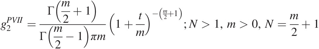
Comparing with the probability density function generator for the bivariate Student t-distribution g2t=πv−1Γv2+1Γv21+tv−v2+1
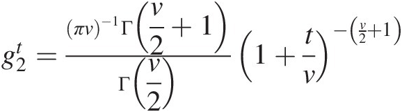 , we show that when N=m2+1
 , the bivariate Pearson type VII distribution reduces to the bivariate Student t-distribution. The same conclusion is reached for higher-dimensional cases.
2. m=1,N=32

When m=1,N=32
 , the probability density function generator of the Pearson type VII distribution may be rewritten as follows:
g2PVIIt=Γ32Γ12π1+t−32,m=1,N=32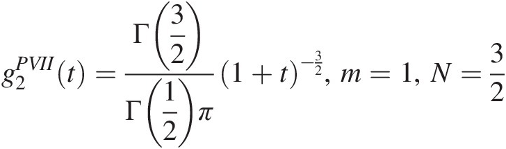
Comparing with the probability density function generation for the Cauchy distribution g2Cauchy=π−1Γ32Γ121+t−32
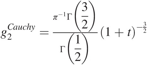 , we show that when m=1,N=32
 , the bivariate Pearson type VII distribution reduces to the bivariate Cauchy distribution. The same conclusion is reached for higher-dimensional cases.


Example 7.6 Compute the Pearson type VII copula density with the information given as follows: m = 0.5, N = 2.0, ρ = 0.1, u = 0.4, v = 0.3m=0.5,N=2.0,ρ=0.1,u=0.4,v=0.3.
Solution: Applying Equation (7.26), we can compute Q−1(u), Q−1(v)Q−1u,Q−1v numerically as follows:
Substituting
Q−1(u) = − 0.1443; Q−1(v) = − 0.3086Q−1u=−0.1443;Q−1v=−0.3086into Equation (7.24), we can compute the copula density function c(0.4, 0.3)c0.40.3 as c(0.4, 0.3) = 1.1941c0.40.3=1.1941.
To illustrate the shape of Pearson type VII distribution, we graph the Pearson type VII copula density function for the following parameters in Figure 7.2:
1. m = 0.5, N = 2.0, ρ = 0.1m=0.5,N=2.0,ρ=0.1.
2. m = 3, N = 2.5, ρ = 0.2m=3,N=2.5,ρ=0.2: bivariate Student t-distribution with degrees of freedom as 3.
3. m=1,N=32,ρ=0.2:
 bivariate Cauchy distribution.


Figure 7.2 Pearson type VII copula density plots.
Symmetric Bivariate Pearson Type II Distribution
The PDF of symmetric bivariate Pearson type II distribution can be expressed as
 (7.28)
where m> − 1m>−1.
The marginal PDF can be given as follows:
 (7.29)
The corresponding CDF can be given as follows:
 (7.30)
The copula probability density function can then be given as follows:
 (7.31)
Example 7.7 Compute the bivariate Pearson type II copula density function with information given as follows: m = − 0.5, ρ = 0.1, u = 0.4, v = 0.3m=−0.5,ρ=0.1,u=0.4,v=0.3.
Solution: Applying Equation (7.30), we can compute Q−1(0.4), Q−1(0.3)Q−10.4,Q−10.3 numerically as follows:
Applying Equation (7.31), we can compute the bivariate Pearson type II copula density function as follows:
To further illustrate the shape of the bivariate Pearson type II copula density function, we graph the Pearson type II copula density function for the following parameters in Figure 7.3:
m = − 0.5, ρ = 0.1m=−0.5,ρ=0.1; (2) m = 0.5, ρ = 0.2m=0.5,ρ=0.2.

Figure 7.3 Pearson type II copula density function plots.
7.2 Two Most Commonly Applied Meta-Elliptical Copulas
In Section 7.1, we have stated that (1) the symmetric meta-Kotz type distribution reduces to the meta-Gaussian distribution if N = s = 1, r = 0.5N=s=1,r=0.5; (2) the symmetric meta-Pearson distribution reduces to the meta-Student t-distribution if N=m2+1 . In this section, we will start to focus on the discussion of two most commonly applied meta-elliptical copulas, and these are meta-Gaussian and meta-Student t copulas.
7.2.1 Meta-Gaussian Copula
A d-dimensional meta-Gaussian copula can be expressed as follows:
 (7.32)
where Φ−1(⋅)Φ−1⋅ represents the inverse function of standard normal distribution; ΦΣ(Φ−1(u1), …., Φ−1(ud))ΦΣΦ−1u1….Φ−1ud represents multivariate standard normal distribution function; ΣΣ represents the correlation matrix; Σ=1⋯ρ1d⋮⋱⋮ρd1⋯1,
ρij=1i=jρjii≠j,ρij=sinπτij2,τi,j the rank correlation coefficient;
d the dimension of continuous multivariate random variables; and w the integral matrix: w = [w1, …, wd]Tw=w1…wdT.
Let gw1…wd=12πd2Σ12exp−12wTΣ−1w,x1=Φ−1u1,…,xd=Φ−1ud , Equation (7.32) may be rewritten as follows:
 (7.32a)
and its copula density function can be given as follows:
 (7.33)
or equivalently
 (7.33a)
Applying the partial derivative rule of inverse function,
 (7.34)
In Equation (7.34), Φ(⋅)Φ⋅ is the CDF of standard normal distribution: Φx=∫−∞x12πe−t22dt ; and ϕ(⋅)ϕ⋅ is the PDF of standard normal distribution: ϕx=12πe−x22
 .
.
Now substituting Equation (7.34) back into Equation (7.32) or (7.32a), we can calculate the partial derivatives for the d-dimensional meta-Gaussian copula in what follows.
First-Order Partial Derivative
Using ∂C∂u1 as an example, the first-order partial derivative of the meta-Gaussian copula may be derived as follows:
 (7.35)
Second-Order Partial Derivative
Using ∂2C∂u1∂u2 as an example, the second-order partial derivative of the meta-Gaussian copula may be derived as follows:
 (7.36)
dth-Order Partial Derivative
Repeating the derivative d-times, we obtain the meta-Gaussian copula density function as follows:
 (7.37)
Let ς = [x1, …, xd]T = [Φ−1(u1), …, Φ−1(ud)]Tς=x1…xdT=Φ−1u1…Φ−1udT. Equation (7.37) may be rewritten as follows:


 (7.38)
Note that in Equation (7.38), ∏i=1de−Φ−1ui22 may be rewritten as follows:
 (7.38a)
 (7.38b)
Substituting Equations (7.38a) and (7.38b) into Equation (7.38), Equation (7.38) may be simplified as follows:
 (7.39)
Recall that ςTς = ςTIςςTς=ςTIς, where I is d by d identity matrix. Equation (7.39) may also be rewritten as follows:
 (7.39a)
Example 7.8 (Bivariate meta-Gaussian copula): Compute the bivariate meta-Gaussian copula and its copula density function with the given information: Σ=10.20.21,u1=0.4,u2=0.3, and show the first-order derivative of the bivariate meta-Gaussian copula.

Solution: Applying Equation (7.32) for d = 2d=2, we have the bivariate meta-Gaussian copula as follows:
 (7.40)
From standard normal distribution, we have the following:

Substituting Φ−1(0.4), Φ−1(0.3), Σ−1Φ−10.4,Φ−10.3,Σ−1 and ∣Σ∣∣Σ∣ into Equation (7.40), we have the following:
Applying Equation (7.39a) for d = 2d=2, we have the meta-Gaussian copula density function as follows:
 (7.40a)
Substituting Φ−1(0.4), Φ−1(0.3), Σ−1Φ−10.4,Φ−10.3,Σ−1 and ∣Σ∣∣Σ∣ into Equation (7.40a), we have the following:
Applying Equation (7.35) for d = 2d=2, we have the first-order derivative of the bivariate meta-Gaussian copula function as follows:
 (7.41)
Substituting Σ=1−ρ2,Σ−1=1−ρ−ρ11−ρ2 into Equation (7.41), we have the following:
 (7.41a)
In Equation (7.41a),
12π∫−∞x2exp−121−ρ2w22−2ρx1w2dw2
may be further simplified as follows:


Let y=w2−ρx11−ρ2 . We have the following:

Finally, Equation (7.41a) is rewritten as follows:
 (7.42)
or equivalently
 (7.42a)
To further illustrate the shape of meta-Gaussian copula and its density function, Figure 7.4 graphs the meta-Gaussian copula and its density function with the use of parameters given in this example.

Figure 7.4 Meta-Gaussian copula and its copula density plots.
Example 7.9 (Trivariate meta-Gaussian copula): compute the trivariate meta-Gaussian copula and its density function.
Compute the copula and its density function with information given as follows:

Also, show the first- and second-order derivatives of the trivariate meta-Gaussian copula.
Applying Equation (7.32) for d = 3d=3, we have the following:
 (7.43)
From standard normal distribution, we have the following:
∣Σ∣∣Σ∣ and Σ−1Σ−1 are calculated as follows:

Integrating Equation (7.43) with the calculated quantity numerically, we have the following:
Applying Equations (7.35) for d = 3d=3, we have the first-order derivative of trivariate meta-Gaussian copula as follows:
 (7.44)
Let Σ=1ρ12ρ13ρ121ρ23ρ13ρ231 , we have the following:

where Σ=1−ρ122−ρ132−ρ232+2ρ12ρ13ρ23
The conditional copula defined in Equation (7.44) follows the bivariate normal distribution that is derived in what follows. Under the condition, i.e., U1 = u1U1=u1 or equivalently X1 = x1X1=x1, we first partition the random variable, ΣΣ, and Σ−1Σ−1 as follows:
 (7.44a)
 (7.44b)
where Σ11=1,Σ12=Σ21T=ρ12ρ13,Σ22=1ρ23ρ231
 (7.44c)
where V11=1Σ1−ρ232,V12=V21T=1∣Σ∣ρ13ρ23−ρ12ρ12ρ23−ρ13

Substituting Equations (7.44a), (7.44b), and (7.44c) into Equation (7.44), we have the following:
 (7.44d)
After some algebra, Equation (7.44d) may be rewritten as follows:
 (7.44e)
where a=−V22−1V21x1,b=x12V11−V21TV22−1V21
Equation (7.44e) can be rewritten as follows:
 (7.44f)
Substituting Equation (7.44f) back into Equation (7.44), we have the following:
 (7.45)
where V22−1=1Σ21−ρ122ρ23−ρ12ρ13ρ23−ρ12ρ131−ρ132 , −V22−1V21x1=1Σρ12×1ρ13×1
 .
.
Similarly, we can derive the second-order derivative of the trivariate meta-Gaussian copula. The second-order derivative of the triavariate meta-Gaussian copula follows the univariate normal distribution, i.e., ∂Cu1u2u3∂u1∂u2~N−x1ρ12ρ23−ρ13+x2ρ12ρ13−ρ231−ρ122Σ1−ρ122 .
.
7.2.2 Meta-Student t Copula
A d-dimensional meta-Student t copula can be expressed as follows:
 (7.46)
where
Tν−1⋅
 represents the inverse of the univariate Student t distribution with νν degrees of freedom.
TΣ,νTν−1u1…Tν−1ud
 represents the multivariate Student t distribution with correlation matrix ΣΣ and νν degrees of freedom in which Σ=1⋯ρ1d⋮⋱⋮ρd1⋯1,ρij=1,i=jρji,i≠j
 .
.
d represents the dimension of variables; and w represents the integral matrix: w = [w1, …, wd]Tw=w1…wdT.


Let gw=Γv+d2Γν21πνd2Σ121+wTΣ−1wν−ν+d2 and x1=Tν−1u1,…xd=Tν−1ud
 . Equation (7.46) can then be rewritten as follows:
 (7.47)
Its copula density function can then be written as follows:
 (7.48)
or equivalently
 (7.48a)
Apply the partial derivative rules of the inverse function:
 (7.49)
Now, substituting Equation (7.49) into Equation (7.48) or (7.48a), we can compute the partial derivatives for the d-dimensional meta-Student t copula. Similar to the d-dimensional meta-Gaussian copula, we will calculate the conditional copula by partitioning the random vector X = [X1, …, Xd]TX=X1…XdT, its correlation matrix ΣΣ, and inverse function Σ−1Σ−1 as follows:
Partitioning X, Σ, Σ−1Σ,Σ−1 as follows:
X=X1X2;Σ=Σ11Σ12Σ21Σ22;Σ−1=V=V11V12V21V22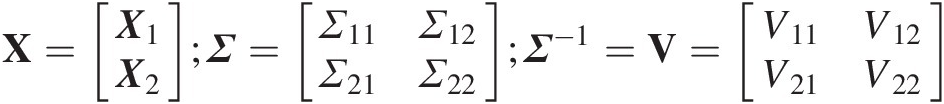 (7.50)

where
X1 = [X1, …, Xd1]TX1=X1…Xd1T (the conditional m-dimensional vector), X2 = [Xd1 + 1, …, Xd]TX2=Xd1+1…XdT; Σ12=Σ21T;V12=V21T ;
;
 (7.50a)
Then, XTΣ−1XXTΣ−1X in Equation (7.48) can be rewritten as follows:

 (7.51)
Expressing the square in X2X2, we can compute the conditional distribution as follows:
where
 (7.51b)
 (7.51c)
Apply the conditional density function fXX1=fXfX1
 ; after some algebra, we have the following:
X ∣ X1~T(X2; μ2 ∣ 1, Σ2 ∣ 1, ν2 ∣ 1)X∣X1~TX2μ2∣1Σ2∣1ν2∣1(7.52)

where
TT represents the multivariate (or univariate) Student t distribution;
 (7.52a)
First-Order Partial Derivative
 (7.53)
In Equation (7.53), gx1w2…wdfx1 is the conditional density function given x1x1. Applying Equations (7.50)–(7.52), we have the conditional copula, which follows the d – 1 cumulative multivariate (or univariate if d = 2) Student t distribution with the following parameters:
 (7.54)
 (7.54b)
Second-Order Partial Derivative
 (7.55)
Similar to the first-order partial derivative for meta-Student t copula, the second-order partial derivative again follows the d-2 cumulative multivariate (or univariate if d = 3) Student t distribution. Based on the derivations given in Equations (7.50)–(7.52), the parameters of the conditional copula are derived in what follows:
Equation (7.50) is rewritten as follows:
 (7.56)
 (7.56a)
Substituting Equation (7.56) back into Equation (7.52), we obtain the parameters for the conditional Student t distribution as follows:
 (7.56c)
 (7.56d)
 (7.56e)
dth-Order Partial Derivative
Using the same approach, the PDF of d-dimensional meta-Student t copula can be obtained as follows:
 (7.57)
Let X=x1…xdT=Tν−1u1…Tν−1udT . Then, g(x1, …, xd)gx1…xd can be given as follows:
 (7.57a)
 (7.57b)
Substituting tνxi=Γν+12Γν2πν121+xi2ν−ν+12 into Equation (7.57b), we have the following:
 (7.57c)
Example 7.10 (Bivariate meta-Student t copula): compute the bivariate meta-Student t copula and its density function.
Compute the copula and its density function with the following information:

Also, show the first-order derivative of the bivariate meta-Student t copula.
Solution: For the bivariate meta-Student t copula, let

and we have the following:


Then, the bivariate meta-Student t copula and its copula density can be expressed as follows:
 (7.58)
 (7.59)
Applying the inverse of univariate Student t distribution with the degrees of freedom (d.f.) = 2, we have the following:

The determinant and the inverse of correlation matrix can be computed as follows:

Substituting the computed quantities into Equation (7.58), we have the following:
Substituting the computed quantities into Equation (7.59), we can compute the copula density function:
c(u1, u2; Σ, ν) = 1.2365cu1u2Σν=1.2365.
Figure 7.5 plots the corresponding copula and its density function.

Figure 7.5 Meta-Student t copula and its density.
In what follows, we give the expression for the first-order derivative of the bivariate meta-Student t distribution.
Applying Equation (7.54a), we have the following:
 (7.60)
 (7.60a)
Substituting Equation (7.60) back into Equation (7.52), we have the following:
 (7.61)
Substituting ν = 2, ρ = 0.2ν=2,ρ=0.2 into Equation (7.61), we have the conditional copula for this example as follows:

Example 7.11 (Trivariate meta-Student t copula): compute the bivariate meta-Student t copula and its density function.
Compute the copula and its density function with the following given information:

Also, show the first- and second-order derivative of the trivariate meta-Student t copula.
Solution: Applying Equation (7.46) for d = 3, we have the following:
 (7.62)
From the Student t distribution with d.f. = 2, we have the following:

|Σ|, Σ−1Σ,Σ−1 can be calculated as follows:

Integrating Equation (7.62) with the computed quantities, we have the following:
In the following, we will show the first- and second-order derivatives of the trivariate meta-Student t copula.
First-order derivative of the trivariate meta-Student t copula:
For the trivariate case, Equation (7.54) can be rewritten for X=X1X2,X1=x1;X2=x2x3 as follows:
 (7.63)
 (7.63a)
 (7.63b)
Substituting Equations (7.63a)–(7.63c) into Equation (7.52), we have the first-order derivative for the trivariate meta-Student t copula as follows:
where BT represents the bivariate cumulative Student t distribution.
Furthermore, for this example, we have the following:


Second-order derivative of the trivariate meta-student t copula:
In this case, Equation (7.56a) can be rewritten for X=X1X2,X1=x1x2;X2=x3 as follows:
 (7.64a)
 (7.64b)
 (7.64c)
Substituting Equations (7.64b)–(7.64d) into Equation (7.52), we have the second-order derivative for the trivariate meta-Student t copula as follows:
Furthermore, for this example, we have the following:


7.3 Parameter Estimation
7.3.1 Marginal Distributions
Marginal CDF of Symmetric Kotz Type Distribution
From qKotz=2srNsπΓNs∫0∞t2+x2N−1exp−rt2+x2sdt , we can use the Gauss–Laguerre numerical integration method to calculate the marginal CDF of the symmetric Kotz type distribution:
 (7.65)
where xixi is the abscissa; ω(xi)ωxi is the weight of abscissas xixi; w(xi)wxi is the total weight of abscissa xixi, w(xi) = ω(xi)exiwxi=ωxiexi; and n is the number of integral nodes. For n = 32, xixi, ω(xi)ωxi and w(xi)wxi are given in Table 7.2.
Table 7.2. Abscissas and weights of Gauss–Laguerre integration.
| No K | Abscissasxixi | Weightω(xi)ωxi | Total weight w(xi)wxi | No K | Abscissas xixi | Weight ω(xi)ωxi | Total weight w(xi)wxi |
|---|---|---|---|---|---|---|---|
| 1 | 0.044489 | 0.109218 | 0.114187 | 17 | 22.63578 | 4.08E–10 | 2.764644 |
| 2 | 0.234526 | 0.210443 | 0.266065 | 18 | 25.62015 | 2.41E–11 | 3.228905 |
| 3 | 0.576885 | 0.235213 | 0.418793 | 19 | 28.87393 | 8.43E–13 | 2.920194 |
| 4 | 1.072449 | 0.195903 | 0.572533 | 20 | 32.33333 | 3.99E–14 | 4.392848 |
| 5 | 1.722409 | 0.129984 | 0.727649 | 21 | 36.1132 | 8.86E–16 | 4.279087 |
| 6 | 2.528337 | 0.070579 | 0.884537 | 22 | 40.13374 | 1.93E–17 | 5.204804 |
| 7 | 3.492213 | 0.031761 | 1.043619 | 23 | 44.52241 | 2.36E–19 | 5.114362 |
| 8 | 4.616457 | 0.011918 | 1.205349 | 24 | 49.20866 | 1.77E–21 | 4.155615 |
| 9 | 5.903958 | 0.003739 | 1.370222 | 25 | 54.35018 | 1.54E–23 | 6.198511 |
| 10 | 7.358127 | 0.000981 | 1.538776 | 26 | 59.87912 | 5.28E–26 | 5.347958 |
| 11 | 8.982941 | 0.000215 | 1.711646 | 27 | 65.98336 | 1.39E–28 | 6.283392 |
| 12 | 10.78301 | 3.92E-05 | 1.889565 | 28 | 72.68427 | 1.87E–31 | 6.891983 |
| 13 | 12.76375 | 5.93E-06 | 2.073189 | 29 | 80.18837 | 1.18E–34 | 7.920911 |
| 14 | 14.93091 | 7.43E-07 | 2.265901 | 30 | 88.73519 | 2.67E–38 | 9.204406 |
| 15 | 17.29327 | 7.63E-08 | 2.469974 | 31 | 98.82955 | 1.34E–42 | 11.16374 |
| 16 | 19.85362 | 6.31E-09 | 2.642967 | 32 | 111.7514 | 4.51E-48 | 15.39024 |
Kotz and Nadarajah (2001) and Nadarajah and Kotz (2005) derived an expression of the hypergeometric function of PDF and CDF of the bivariate symmetric Kotz type distribution and a marginal CDF of the bivariate Pearson type II and VII distributions in the incomplete beta function, respectively.
The PDF and CDF of the bivariate symmetric Kotz type distribution, for z>0z>0, are
 (7.66)
where ψψ is the degenerate hypergeometric function given as follows:
 (7.66a)
 (7.66b)
 (7.66c)
The corresponding CDF for z>0z>0
 (7.67)
where
 (7.67a)
Equation (7.67) needs to satisfy Ns−is−12s+1≠0 and Ns+1≠0
 .
.
Since Equation (7.67) is an expression of hypergeometric function, it needs to satisfy Ns−is−12s+1≠0 , and the numerical solution may experience overflow. Therefore, the Gauss–Laguerre integration and multiple complex Gauss–Legendre integral formulae can be used to compute the marginal PDF and CDF of bivariate symmetric Kotz type distribution, respectively.
For the marginal PDF, the Gauss–Laguerre integration can be used as
 (7.68)
where tktk and w(tk)wtk are the abscissa and the weight of the Gauss–Laguerre integration, respectively; m is the integral node; and q is the node of Gauss–Legendre integration. For CDF, we use multiple complex Gauss–Legendre integral formulae (Zhang, 2000):
 (7.69)
where q is the node of Gauss–Legendre integration; a, b are the upper and lower integral limits of variable x; ψ(x) and φ(x)ψxandφx are the upper and lower integral limits of variable y; and m is a positive integer that breaks the interval [a, b] of x into m equal pieces. The width of each piece is Δx=b−am;xj=a+jΔx,j=0,1,…,m;x˜ji=xj+Δx21+x˜iq , x˜iq
 is the abscissa of ith node of the Gauss–Legendre integration; and njnj is a positive integer that breaks the interval φx˜jiψx˜ji
 of yy into njnj equal pieces, Δyj=ψx˜ji−φx˜jinj;
yl=φx˜ji+lΔyj,l=0,1,…,nj;y˜lk=yl+1+x˜kqΔyj2 ; αiqandβq
 are the abscissas of the ith and kth nodes of the Gauss–Legendre and the Gauss–Laguerre integration, respectively; x˜kq
 is the abscissa of the kth node of the Gauss–Laguerre integration. From Equation (7.69), we know the integral interval is [0, ∞)0∞. Using the Gauss–Laguerre integration for y, one can get
 (7.70)
Marginal CDF of Symmetric Pearson Type VII Distribution
According to Fang et al. (2002), for z = [x, y]z=xy the bivariate symmetric Pearson type VII distribution can be given as follows:
 (7.71)
Through integration, the marginal CDF of the symmetric Pearson type VII distribution can be written as follows:
 (7.72)
On one hand, Equation (7.72) can be solve by applying the Gauss–Laguerre integration to compute the marginal CDF; on the other hand, it can be solved by applying the incomplete beta function (Kotz and Nadarajah, 2001), as follows:
 (7.73)
where Ix(a, b)Ixab is the incomplete beta function, as follows:
 (7.73a)
 (7.73b)
Results of the Gauss–Laguerre integration and incomplete beta function results by Kotz and Nadarajah (2001) are very close, as shown in Table 7.3.
Table 7.3. Marginal CDF of the symmetric Pearson type VII distribution (N = 4.0; m = 5.5)
| xx | qp7(x)qp7x | Qp7(x)[1]Qp7x1 | Qp7(x)[2]Qp7x2 | xx | qp7(x)qp7x | Qp7(x)[1]Qp7x1 | Qp7(x)[2]Qp7x2 |
|---|---|---|---|---|---|---|---|
| −3.0 | 0.0134 | 0.0101 | 0.0101 | 0.0 | 0.3998 | 0.5000 | 0.5000 |
| −2.9 | 0.0155 | 0.0116 | 0.0116 | 0.1 | 0.3972 | 0.5399 | 0.5399 |
| −2.8 | 0.0180 | 0.0132 | 0.0132 | 0.2 | 0.3897 | 0.5793 | 0.5793 |
| −2.7 | 0.0208 | 0.0152 | 0.0152 | 0.3 | 0.3777 | 0.6177 | 0.6177 |
| −2.6 | 0.0242 | 0.0174 | 0.0174 | 0.4 | 0.3616 | 0.6547 | 0.6547 |
| −2.5 | 0.0280 | 0.0200 | 0.0200 | 0.5 | 0.3422 | 0.6899 | 0.6899 |
| −2.4 | 0.0326 | 0.0231 | 0.0231 | 0.6 | 0.3202 | 0.7230 | 0.7230 |
| −2.3 | 0.0378 | 0.0266 | 0.0266 | 0.7 | 0.2965 | 0.7539 | 0.7539 |
| −2.2 | 0.0439 | 0.0306 | 0.0306 | 0.8 | 0.2719 | 0.7823 | 0.7823 |
| −2.1 | 0.0509 | 0.0354 | 0.0354 | 0.9 | 0.2471 | 0.8083 | 0.8083 |
| −2.0 | 0.0590 | 0.0409 | 0.0409 | 1.0 | 0.2228 | 0.8317 | 0.8317 |
| −1.9 | 0.0684 | 0.0472 | 0.0472 | 1.1 | 0.1993 | 0.8528 | 0.8528 |
| −1.8 | 0.0790 | 0.0546 | 0.0546 | 1.2 | 0.1771 | 0.8716 | 0.8716 |
| −1.7 | 0.0912 | 0.0631 | 0.0631 | 1.3 | 0.1565 | 0.8883 | 0.8883 |
| −1.6 | 0.1049 | 0.0729 | 0.0729 | 1.4 | 0.1376 | 0.9030 | 0.9030 |
| −1.5 | 0.1204 | 0.0841 | 0.0841 | 1.5 | 0.1204 | 0.9159 | 0.9159 |
| −1.4 | 0.1376 | 0.0970 | 0.0970 | 1.6 | 0.1049 | 0.9271 | 0.9271 |
| −1.3 | 0.1565 | 0.1117 | 0.1117 | 1.7 | 0.0912 | 0.9369 | 0.9369 |
| −1.2 | 0.1771 | 0.1284 | 0.1284 | 1.8 | 0.0790 | 0.9454 | 0.9454 |
| −1.1 | 0.1993 | 0.1472 | 0.1472 | 1.9 | 0.0684 | 0.9528 | 0.9528 |
| −1.0 | 0.2228 | 0.1683 | 0.1683 | 2.0 | 0.0590 | 0.9591 | 0.9591 |
| −0.9 | 0.2471 | 0.1917 | 0.1917 | 2.1 | 0.0509 | 0.9646 | 0.9646 |
| −0.8 | 0.2719 | 0.2177 | 0.2177 | 2.2 | 0.0439 | 0.9694 | 0.9694 |
| −0.7 | 0.2965 | 0.2461 | 0.2461 | 2.3 | 0.0378 | 0.9734 | 0.9734 |
| −0.6 | 0.3202 | 0.2770 | 0.2770 | 2.4 | 0.0326 | 0.9769 | 0.9769 |
| −0.5 | 0.3422 | 0.3101 | 0.3101 | 2.5 | 0.0280 | 0.9800 | 0.9800 |
| −0.4 | 0.3616 | 0.3453 | 0.3453 | 2.6 | 0.0242 | 0.9826 | 0.9826 |
| −0.3 | 0.3777 | 0.3823 | 0.3823 | 2.7 | 0.0208 | 0.9848 | 0.9848 |
| −0.2 | 0.3897 | 0.4207 | 0.4207 | 2.8 | 0.0180 | 0.9868 | 0.9868 |
| −0.1 | 0.3972 | 0.4601 | 0.4601 | 2.9 | 0.0155 | 0.9884 | 0.9884 |
Note: QPVII(x)[1]QPVIIx1 : Gauss–Laguerre integration; QPVII(x)[2]QPVIIx2: Kotz and Nadarajah (2001).
Its bivariate copula density can be given as follows:
 (7.74)
where x=Qp7−1u,y=Qp7−1v .
.
Marginal CDF of Symmetric Pearson Type II Distribution
Again, based on Fang et al. (2002), the probability density function of symmetric bivariate Pearson II distribution (for z = [x, y]z=xy) can be given as follows:
 (7.75)
The marginal CDF of symmetric Pearson type II distribution can be expressed as follows:
 (7.76)
Applying the Gauss–Legendre integration method, we can compute the marginal CDF of the symmetric Pearson type II distribution using the following:
 (7.77)
Table 7.4 lists the abscissa and the weight of the Gauss–Legendre integration.
Table 7.4. Abscissa and weight of the Gauss–Legendre integration.
| No k | Abscissa xkxk | Weight ω(xk)ωxk | No K | Abscissa xkxk | Weight ω(xk)ωxk |
|---|---|---|---|---|---|
| 1 | 0.99726 | 0.007018 | 17 | 0.048308 | 0.09654 |
| 2 | −0.98561 | 0.016277 | 18 | 0.144472 | 0.095638 |
| 3 | −0.96476 | 0.025391 | 19 | 0.239287 | 0.093844 |
| 4 | −0.93491 | 0.034275 | 20 | 0.331869 | 0.091174 |
| 5 | −0.89632 | 0.042836 | 21 | 0.421351 | 0.087652 |
| 6 | −0.84937 | 0.050998 | 22 | 0.5069 | 0.083312 |
| 7 | −0.79448 | 0.058684 | 23 | 0.587716 | 0.078194 |
| 8 | −0.73218 | 0.065822 | 24 | 0.663044 | 0.072346 |
| 9 | −0.66304 | 0.072346 | 25 | 0.732182 | 0.065822 |
| 10 | −0.58772 | 0.078194 | 26 | 0.794484 | 0.058684 |
| 11 | −0.5069 | 0.083312 | 27 | 0.849368 | 0.050998 |
| 12 | −0.42135 | 0.087652 | 28 | 0.896321 | 0.042836 |
| 13 | −0.33187 | 0.091174 | 29 | 0.934906 | 0.034275 |
| 14 | −0.23929 | 0.093844 | 30 | 0.964762 | 0.025391 |
| 15 | −0.14447 | 0.095638 | 31 | 0.985612 | 0.016277 |
| 16 | −0.04831 | 0.09654 | 32 | 0.997264 | 0.007018 |
Similar to the marginal CDF of the symmetric Pearson Type VII distribution, the marginal CDF of symmetric Pearson type II distribution may be solved using the incomplete beta function as follows:
 (7.78)
Comparing the equation of incomplete beta function given by Kotz and Nadarajah (2001), the marginal CDFs computed from the two methods with the given parameter m are very close, as shown in Table 7.5.
Table 7.5. Marginal CDF of symmetric Pearson type II distribution (m = 4.5).
| xx | qp2(x)qp2x | Qp2(x)Qp2x[1] | Qp2(x)Qp2x[2] | xx | qp2(x)qp2x | Qp2(x)Qp2x[1] | Qp2(x)Qp2x[2] |
|---|---|---|---|---|---|---|---|
| –1.0 | 0.0000 | 0.0000 | 0.0000 | 0.0 | 1.3535 | 0.5000 | 0.5000 |
| –0.9 | 0.0003 | 0.0000 | 0.0000 | 0.1 | 1.2872 | 0.6331 | 0.6331 |
| –0.8 | 0.0082 | 0.0003 | 0.0003 | 0.2 | 1.1036 | 0.7535 | 0.7535 |
| –0.7 | 0.0467 | 0.0027 | 0.0027 | 0.3 | 0.8446 | 0.8513 | 0.8513 |
| –0.6 | 0.1453 | 0.0117 | 0.0117 | 0.4 | 0.5661 | 0.9218 | 0.9218 |
| –0.5 | 0.3212 | 0.0343 | 0.0343 | 0.5 | 0.3212 | 0.9657 | 0.9657 |
| –0.4 | 0.5661 | 0.0782 | 0.0782 | 0.6 | 0.1453 | 0.9883 | 0.9883 |
| –0.3 | 0.8446 | 0.1487 | 0.1487 | 0.7 | 0.0467 | 0.9973 | 0.9973 |
| –0.2 | 1.1036 | 0.2465 | 0.2465 | 0.8 | 0.0082 | 0.9997 | 0.9997 |
| –0.1 | 1.2872 | 0.3669 | 0.3669 | 0.9 | 0.0003 | 1.0000 | 1.0000 |
Note: Qp2(x)Qp2x[1]: Gauss–Legendre integration; Qp2(x)Qp2x[2]: Kotz and Nadarajah (2001).
7.3.2 Parameter Estimation
Generally speaking, the pseudo-maximum likelihood method may still be used to estimate parameters of meta-elliptical copulas (Nadarajah and Kotz, 2005). Here we will first introduce the pseudo-maximum likelihood function for Kotz and Pearson type meta-elliptical copulas. Then, we again focus on meta-Gaussian and meta-Student t copulas with examples.
Bivariate Symmetric Kotz Type Distribution
The joint probability density function of the bivariate symmetric Kotz type distribution can be given as follows:
 (7.79)
Then, the log-likelihood function can be given as follows:
 (7.79a)
Taking the first-order derivative of Equation (7.79a) with respect to parameters N, r, s, ρN,r,s,ρ, we have the following:
 (7.79b)
Bivariate Pearson Type VII Distribution
The log-likelihood function of the bivariate Pearson type VII distribution [Equation (7.71)] can be written as:
 (7.80)
Taking the first-order derivative of Equation (7.80) with respect to parameters N, m, ρN,m,ρ, we have the following:
 (7.80a)
Bivariate Pearson Type II Distribution
The log-likelihood function of the bivariate Pearson type II distribution (Equation (7.75)) can be written as follows:
 (7.81)
Taking the first-order derivative of Equation (7.81) with respect to parameters m, ρm,ρ, we have the following:
 (7.81a)
Setting Equations (7.79b), (7.80a), and (7.81a) to 0, we can estimate the parameters of the bivariate Kotz, Pearson VII, and Pearson II distributions by solving these equations simultaneously.
Example 7.12 Estimation of parameters of meta-Gaussian copula with the data given in Table 7.6.
Table 7.6. Three-dimensional data sample.
| No. | u1u1 | u2u2 | u3u3 | No. | u1u1 | u2u2 | u3u3 |
|---|---|---|---|---|---|---|---|
| 1 | 0.8085 | 0.4026 | 0.7069 | 26 | 0.8044 | 0.3380 | 0.9206 |
| 2 | 0.8845 | 0.9449 | 0.9775 | 27 | 0.8441 | 0.3217 | 0.7441 |
| 3 | 0.0483 | 0.0201 | 0.0259 | 28 | 0.3713 | 0.5469 | 0.3967 |
| 4 | 0.5818 | 0.4478 | 0.7189 | 29 | 0.8165 | 0.5460 | 0.6650 |
| 5 | 0.7066 | 0.6085 | 0.6556 | 30 | 0.0444 | 0.2351 | 0.2073 |
| 6 | 0.0543 | 0.5992 | 0.0555 | 31 | 0.6413 | 0.8358 | 0.7090 |
| 7 | 0.4799 | 0.3308 | 0.4113 | 32 | 0.0675 | 0.2407 | 0.1012 |
| 8 | 0.7468 | 0.6777 | 0.6236 | 33 | 0.0142 | 0.1737 | 0.0638 |
| 9 | 0.9989 | 0.9913 | 0.9984 | 34 | 0.3875 | 0.7339 | 0.1912 |
| 10 | 0.9353 | 0.9649 | 0.9661 | 35 | 0.0237 | 0.0136 | 0.0091 |
| 11 | 0.0002 | 0.0012 | 0.0033 | 36 | 0.7743 | 0.8217 | 0.8119 |
| 12 | 0.9388 | 0.9533 | 0.9835 | 37 | 0.2967 | 0.8092 | 0.6397 |
| 13 | 0.8777 | 0.7798 | 0.7347 | 38 | 0.5267 | 0.2084 | 0.1927 |
| 14 | 0.2764 | 0.7564 | 0.4758 | 39 | 0.8736 | 0.8376 | 0.8816 |
| 15 | 0.8212 | 0.8777 | 0.7088 | 40 | 0.0968 | 0.0587 | 0.0861 |
| 16 | 0.4701 | 0.4711 | 0.4284 | 41 | 0.4120 | 0.0877 | 0.4317 |
| 17 | 0.7744 | 0.1112 | 0.4433 | 42 | 0.3236 | 0.4496 | 0.3733 |
| 18 | 0.4937 | 0.6475 | 0.8518 | 43 | 0.2043 | 0.7927 | 0.6416 |
| 19 | 0.7424 | 0.5635 | 0.8267 | 44 | 0.5628 | 0.9067 | 0.5870 |
| 20 | 0.7120 | 0.9838 | 0.9100 | 45 | 0.1844 | 0.2117 | 0.2585 |
| 21 | 0.9757 | 0.5134 | 0.7641 | 46 | 0.2724 | 0.5463 | 0.4876 |
| 22 | 0.3326 | 0.3769 | 0.1272 | 47 | 0.0737 | 0.3664 | 0.3733 |
| 23 | 0.8493 | 0.6129 | 0.7113 | 48 | 0.5192 | 0.2766 | 0.6553 |
| 24 | 0.7328 | 0.9191 | 0.9038 | 49 | 0.3644 | 0.6738 | 0.8504 |
| 25 | 0.5228 | 0.4322 | 0.6576 | 50 | 0.9005 | 0.3035 | 0.8588 |
Solution: Let {x1i, x2i, …, xdi}x1ix2i…xdi be a d-dimensional sample where i = 1, …, n, u1i = F1(x1i), …, udi = Fd(xdi)i=1,…,n,u1i=F1x1i,…,udi=Fdxdi. The parameter space is denoted as θ = {Σ : Σ ∈ Ω}θ=Σ:Σ∈Ω, where ΣΣ is symmetric and a positive definite matrix. Applying Equation (7.39a), the log-likelihood function of the d-dimensional meta-Gaussian copula can be written as follows:

 (7.82)
where ξi = [x1i, …, xdi]T = [Φ−1(u1i), …., Φ−1(udi)]Tξi=x1i…xdiT=Φ−1u1i….Φ−1udiT; tr(⋅)tr⋅ trace of the matrix.
Assuming Equation (7.82) is differentiable in θθ, parameters of the meta-Gaussian copula can be solved for by ∂logL∂θ=0 as follows:
 (7.82a)
From Equation (7.82a), we have the following:
 (7.82b)
To estimate the parameters (i.e., covariance matrix) of the meta-Gaussian copula, we first need to compute ξi = [Φ−1(u1i), Φ−1(u2i), Φ−1(u3i)]; Φ(⋅) : inverse of N(0, 1),ξi=Φ−1u1iΦ−1u2iΦ−1u3i;Φ⋅:inverse ofN01, as shown in Table 7.7.
Table 7.7. Inverse normal distribution: N(0,1).
| No. | u1u1 | u2u2 | u3u3 | Φ−1(u1)Φ−1u1 | Φ−1(u2)Φ−1u2 | Φ−1(u3)Φ−1u3 |
|---|---|---|---|---|---|---|
| 1 | 0.8085 | 0.4026 | 0.7069 | 0.8723 | –0.2466 | 0.5444 |
| 2 | 0.8845 | 0.9449 | 0.9775 | 1.1977 | 1.5976 | 2.0040 |
| 3 | 0.0483 | 0.0201 | 0.0259 | –1.6612 | –2.0523 | –1.9443 |
| 4 | 0.5818 | 0.4478 | 0.7189 | 0.2064 | –0.1311 | 0.5797 |
| 5 | 0.7066 | 0.6085 | 0.6556 | 0.5435 | 0.2754 | 0.4004 |
| 6 | 0.0543 | 0.5992 | 0.0555 | –1.6046 | 0.2512 | –1.5941 |
| 7 | 0.4799 | 0.3308 | 0.4113 | –0.0504 | –0.4378 | –0.2242 |
| 8 | 0.7468 | 0.6777 | 0.6236 | 0.6643 | 0.4613 | 0.3149 |
| 9 | 0.9989 | 0.9913 | 0.9984 | 3.0622 | 2.3775 | 2.9566 |
| 10 | 0.9353 | 0.9649 | 0.9661 | 1.5163 | 1.8109 | 1.8264 |
| 11 | 0.0002 | 0.0012 | 0.0033 | –3.4847 | –3.0458 | –2.7162 |
| 12 | 0.9388 | 0.9533 | 0.9835 | 1.5446 | 1.6775 | 2.1332 |
| 13 | 0.8777 | 0.7798 | 0.7347 | 1.1638 | 0.7714 | 0.6271 |
| 14 | 0.2764 | 0.7564 | 0.4758 | –0.5935 | 0.6947 | –0.0606 |
| 15 | 0.8212 | 0.8777 | 0.7088 | 0.9201 | 1.1633 | 0.5499 |
| 16 | 0.4701 | 0.4711 | 0.4284 | –0.0750 | –0.0724 | –0.1805 |
| 17 | 0.7744 | 0.1112 | 0.4433 | 0.7533 | –1.2202 | –0.1427 |
| 18 | 0.4937 | 0.6475 | 0.8518 | -0.0158 | 0.3787 | 1.0442 |
| 19 | 0.7424 | 0.5635 | 0.8267 | 0.6508 | 0.1598 | 0.9411 |
| 20 | 0.7120 | 0.9838 | 0.9100 | 0.5593 | 2.1394 | 1.3409 |
| 21 | 0.9757 | 0.5134 | 0.7641 | 1.9729 | 0.0335 | 0.7197 |
| 22 | 0.3326 | 0.3769 | 0.1272 | –0.4328 | –0.3137 | –1.1396 |
| 23 | 0.8493 | 0.6129 | 0.7113 | 1.0332 | 0.2869 | 0.5573 |
| 24 | 0.7328 | 0.9191 | 0.9038 | 0.6213 | 1.3990 | 1.3035 |
| 25 | 0.5228 | 0.4322 | 0.6576 | 0.0573 | –0.1707 | 0.4060 |
| 26 | 0.8044 | 0.3380 | 0.9206 | 0.8574 | –0.4179 | 1.4092 |
| 27 | 0.8441 | 0.3217 | 0.7441 | 1.0114 | –0.4630 | 0.6561 |
| 28 | 0.3713 | 0.5469 | 0.3967 | –0.3284 | 0.1179 | –0.2619 |
| 29 | 0.8165 | 0.5460 | 0.6650 | 0.9022 | 0.1157 | 0.4262 |
| 30 | 0.0444 | 0.2351 | 0.2073 | –1.7019 | –0.7221 | –0.8160 |
| 31 | 0.6413 | 0.8358 | 0.7090 | 0.3620 | 0.9773 | 0.5504 |
| 32 | 0.0675 | 0.2407 | 0.1012 | –1.4947 | –0.7041 | –1.2746 |
| 33 | 0.0142 | 0.1737 | 0.0638 | –2.1916 | –0.9396 | –1.5240 |
| 34 | 0.3875 | 0.7339 | 0.1912 | –0.2859 | 0.6248 | –0.8735 |
| 35 | 0.0237 | 0.0136 | 0.0091 | –1.9832 | –2.2086 | –2.3609 |
| 36 | 0.7743 | 0.8217 | 0.8119 | 0.7532 | 0.9220 | 0.8849 |
| 37 | 0.2967 | 0.8092 | 0.6397 | –0.5340 | 0.8749 | 0.3576 |
| 38 | 0.5267 | 0.2084 | 0.1927 | 0.0670 | –0.8120 | –0.8681 |
| 39 | 0.8736 | 0.8376 | 0.8816 | 1.1436 | 0.9848 | 1.1832 |
| 40 | 0.0968 | 0.0587 | 0.0861 | –1.2999 | –1.5657 | –1.3654 |
| 41 | 0.4120 | 0.0877 | 0.4317 | –0.2224 | –1.3549 | –0.1719 |
| 42 | 0.3236 | 0.4496 | 0.3733 | –0.4576 | –0.1266 | –0.3232 |
| 43 | 0.2043 | 0.7927 | 0.6416 | –0.8265 | 0.8157 | 0.3627 |
| 44 | 0.5628 | 0.9067 | 0.5870 | 0.1580 | 1.3205 | 0.2199 |
| 45 | 0.1844 | 0.2117 | 0.2585 | –0.8989 | –0.8005 | –0.6479 |
| 46 | 0.2724 | 0.5463 | 0.4876 | –0.6056 | 0.1163 | –0.0310 |
| 47 | 0.0737 | 0.3664 | 0.3733 | –1.4490 | –0.3413 | –0.3231 |
| 48 | 0.5192 | 0.2766 | 0.6553 | 0.0483 | –0.5928 | 0.3996 |
| 49 | 0.3644 | 0.6738 | 0.8504 | –0.3468 | 0.4504 | 1.0383 |
| 50 | 0.9005 | 0.3035 | 0.8588 | 1.2842 | –0.5143 | 1.0749 |
Applying Equation (7.82b), we have Σ=10.67000.87580.670010.79450.87580.79451 .
.
Example 7.13 Show how to estimate parameters of the meta-Student t copula.
Let {x1i, x2i, …, xdi}x1ix2i…xdi be a d-dimensional sample where i = 1, …, n, u1i = F1(x1i), …, udi = Fd(xdi)i=1,…,n,u1i=F1x1i,…,udi=Fdxdi. In the case of meta-Student t copula, its parameter space is θ = {(ν, Σ) : ν ∈ (1, ∞), Σ ∈ Ω }θ=νΣ:ν∈1∞Σ∈Ω. In the same way as in the meta-Gaussian copula, ΣΣ is symmetric and positive definite. Applying the meta-Student t copula density function (i.e., Equation (7.57)), the log-likelihood function can be given as follows:
 (7.83)
where ξi=Tν−1u1i…Tν−1udiT , and νν is the degree of freedom.
To estimate the fitted parameters θ̂=ν̂Σ̂ , we may apply the following two approaches:
1. Optimizing the log-likelihood function (Equation (7.83)) numerically with the constraint of ΣΣ being symmetric and with ones on the main diagonal. With this constraint, the MLE estimate of Σ̂
 may not be positive and semidefinite.
2. Estimate Σ̂
 and νν separately.
Σ̂
 may be estimated from the sample Kendall tau using the following:
τ̂UiUj=2πarcsinρ̂ij⇒ρ̂ij=sinπ2τ̂ij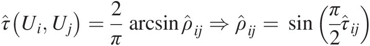 (7.84)
where τ̂ij=τ̂UiUj
 is the sample Kendall tau between random variable UiUi and UjUj; and ρ̂ij
 is the off-diagonal element of correlation matrix ΣΣ. In the same way as in approach 1, the estimated correlation matrix may not be positive definite.
Estimate the single parameter νν using MLE (Equation (7.83)) by fixing Σ̂
 .
.


For the estimated Σ̂ not being positive and semidefinite, we can apply the procedure discussed by McNeil et al. (2005) to convert it into positive definite matrix with the procedure as follows:
i. Compute the eigenvalue decomposition Σ = EDETΣ=EDET, where E is an orthogonal matrix that contains eigenvectors, and D is the diagonal matrix that contains all the eigenvalues.
ii. Construct a diagonal matrix D˜
 by replacing all negative eigenvalues in D by a small value δ>0δ>0.
iii. Compute Σ˜=ED˜ET
 , Σ˜
, Σ˜ is positive definite but not necessarily a correlation matrix.
iv. Apply the normalizing operator P
 to obtain the desired correlation matrix.


Specifically, for the bivariate case, the parameters that need to be estimated are θ = (ρ, ν)θ=ρν. Thus, the log-likelihood function (i.e., Equation (7.83)) can be rewritten as follows:
 (7.85)
Taking the first-order derivative with respect to ρ, ν,ρ,ν, we have the following:
 (7.85a)
 (7.85b)
Example 7.14 Using the data given in Table 7.7, estimate the parameters for the bivariate (using u1, u2)u1,u2) and the trivariate meta-Student t copula.
Solution:
Bivariate meta-Student t copula (using u1, u2)u1,u2)
Approach 1
For the bivariate case, we will apply Equation (7.85), i.e., maximizing the bivariate meta-Student t log-likelihood function.
The initial correlation coefficient is set as the sample correlation coefficient computed from the sample Kendall tau (τ̂0=0.3812
 ) using Equation (7.84) as follows:
ρ̂0=sinπ2τ̂0=sin0.3812π2=0.5637.
The initial degree of freedom (d.f.) is set as the lower limit (i.e., ν̂0=10
 ).
).
Then, the final parameter set θ̂=ρ̂ν̂:ρ∈−11ν>1
 may be estimated using the optimization toolbox (e.g., the fmincon function) by minimizing the negative log-likelihood function (the objective function), which is the dual problem of the MLE estimation. We have the following:
θ̂=ρ̂ν̂=0.55916.2531
 . With the estimated correlation coefficient, the correlation matrix is given as follows: Σ=10.55910.55911
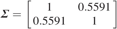 . The eigenvalue of the correlation matrix is λ=0.44091.5591
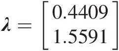 , i.e., the correlation matrix is positive definite.
Furthermore, one can use the MATLAB function copulafit to estimate the parameters of the meta-Student t copula using the MLE method. The function is given as follows:
MLE: Σ̂ν̂=copulafit’t’data
Using MLE from MATLAB, we have the following:
Σ̂=10.55910.55911,ν̂=6.2542.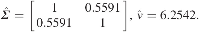
Approach 2
Fixing ρ̂=0.5637
 , we haveν̂=6.4110
 .
.


Trivariate meta-Student t copula
Approach 1
It is shown for the bivariate case that the parameters estimated using the embedded MATLAB function and those estimated using the fmincon by writing our own objective function are almost the same. So for the trivariate example, we will only show the results obtained from the embedded MATLAB function.
Applying approach 1 and maximizing the log-likelihood function of the trivariate meta-Student t copula, using the embedded MATLAB function mentioned previously, we have the following ML method:
Σ̂=10.58310.81710.583110.75180.81710.75181,ν̂=12.8139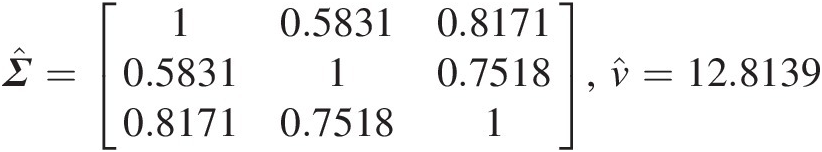
Approach 2
To apply approach 2, we first need to compute the sample correlation matrix from the sample Kendall tau using Equation (7.84) as follows:
τ=10.38120.65880.381210.51020.65880.51021,Σ=10.56370.85980.563710.71830.85980.71831.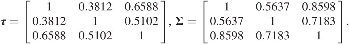
The eigenvalue vector of ΣΣ is computed as λ = [0.1116, 0.4537, 2.4347]Tλ=0.11160.45372.4347T. Thus, we reach the conclusion that the correlation matrix is positive definite.
Fixing the correlation matrix ΣΣ, we only have one parameter, i.e., νν, that needs to be estimated. Optimizing the log-likelihood equation (i.e., Equation (7.83)), we can estimate νν with an initial estimate of ν̂0=2
 . Using the fmincon function, we have ν̂=20.4038
 .
.
It should be noted here for the meta-Student t copula that one can also use the following embedded function: Σ̂ν̂=copulafit’t’data,’Method’,’ApproximateML’.
 This estimation method is considered as a good estimation only if the sample size is large enough.


7.4 Summary
In this chapter, we have summarized and discussed the properties of meta-elliptical copulas. We have explained the procedures on how to construct and apply the meta-elliptical copulas, especially for the meta-Gaussian and meta-Student t copulas. Comparing meta-Gaussian and meta-Student t copulas, both copulas may be applied to model the dependence of entire range. The Student t copula possesses the symmetric upper (lower) tail dependence, while the meta-Gaussian copula does not possess the tail dependence. The meta-elliptical copula may be applied for the multivariate frequency analysis.