Abstract
The stratospheric ozone layer results from the photolysis of molecular oxygen by ultraviolet (UV) solar radiation in the high atmosphere. This large atmospheric layer is stable and, therefore, affects the general atmospheric circulation by decreasing significantly the vertical motions of air parcels. In addition, ozone protects the Earth from harmful UV radiation. Therefore, its destruction by anthropogenic activities may lead to public health impacts. This chapter presents first some fundamentals of atmospheric chemical kinetics (i.e., the speed at which chemical reactions occur in the atmosphere), which are needed to understand the processes leading to the presence of the ozone layer. These notions are also needed to understand the formation of gaseous and particulate pollutants, which is presented in the following chapters. Next, the processes that govern the ozone layer are described in terms of its natural formation and its destruction by man-made substances. Finally, the public policies introduced to address the protection of the stratospheric ozone layer are summarized.
The stratospheric ozone layer results from the photolysis of molecular oxygen by ultraviolet (UV) solar radiation in the high atmosphere. This large atmospheric layer is stable and, therefore, affects the general atmospheric circulation by decreasing significantly the vertical motions of air parcels. In addition, ozone protects the Earth from harmful UV radiation. Therefore, its destruction by anthropogenic activities may lead to public health impacts. This chapter presents first some fundamentals of atmospheric chemical kinetics (i.e., the speed at which chemical reactions occur in the atmosphere), which are needed to understand the processes leading to the presence of the ozone layer. These notions are also needed to understand the formation of gaseous and particulate pollutants, which is presented in the following chapters. Next, the processes that govern the ozone layer are described in terms of its natural formation and its destruction by man-made substances. Finally, the public policies introduced to address the protection of the stratospheric ozone layer are summarized.
7.1 Fundamentals of Chemical Kinetics
7.1.1 Atmospheric Concentration Units
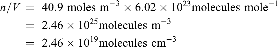
The ideal gas law was shown in Chapter 4 to apply to the atmosphere. Therefore, at an atmospheric pressure P = 1 atm, i.e., at sea level, and a temperature T = 298 K (i.e., 25 °C), the air contains 40.9 moles m−3. Atmospheric concentrations may be expressed in various units, and the following ones are generally used in atmospheric chemistry:
– Moles per unit volume of air
– Molecules per unit volume of air
– Molar fraction (also called mixing ratio)
– Mass per unit volume of air
The conversion of moles per unit volume of air into molecules per unit volume of air is done using the Avogadro number, N, which is the number of molecules per mole (N = 6.02 × 10²³ molecules mole−1).
There are 40.9 moles of air per m3 at 1 atm and 25 °C, therefore:
 (7.1)
(7.1) Molecular concentrations are usually given in molecules per cm3 (i.e., molec cm−3).
The molar fraction (also referred to as mixing ratio) is the ratio of the number of moles (or molecules) of a chemical species and of the number of moles (or molecules) of air (i.e., nitrogen + oxygen + argon + other minor constituents). Therefore, the molar fraction of pure air is 1. For a gaseous pollutant, it is of course much less than 1. Accordingly, the molar fraction is usually expressed as ppm (parts per million), ppb (parts per billion), or ppt (parts per trillion). If there is a molecule of a chemical species per million molecules of air, its molar fraction is 1 ppm. If there is a molecule of a chemical species per billion molecules of air, its molar fraction is 1 ppb. The molar fraction of pure air is by definition 106 ppm, i.e., 109 ppb, or 1012 ppt.
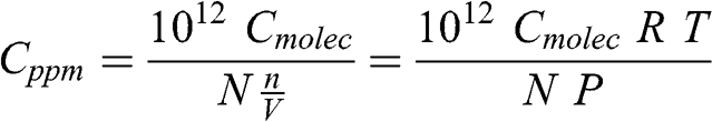
The conversion of the molar (or molecular) concentration of a species into a molar fraction (or vice versa) is done using the ideal gas law. Therefore, this conversion depends on pressure and temperature. For example, let Cmolec be the molecular concentration expressed in molec cm−3. The molar fraction expressed in ppm, Cppm, is calculated as follows (V is expressed here in m3):
 (7.2)
(7.2) where R = 8.206 × 10⁻⁵ atm m3 mole−1 K−1. If a chemical species is uniformly mixed within the atmosphere, its molar fraction is constant. On the other hand, its molar or molecular concentration decreases with altitude, since pressure decreases with altitude (temperature also decreases with altitude in the troposphere, but the absolute temperature gradient is less than the pressure gradient).
The mass concentration is derived from the molar concentration (or from the molecular concentration) using the molar mass of the chemical species, MM. Let Cmass be the mass concentration of a chemical species (expressed here in μg m−3). It is calculated from the molecular concentration, Cmolec (expressed here in molec cm−3), as follows:
 (7.3)
(7.3) where the factor 1012 corresponds to conversions from g to μg and from cm3 to m3.
The conversion of the mass concentration into molar fraction (or vice versa) is done using the ideal gas law and, therefore, depends on pressure and temperature. For example, to obtain the molar fraction in ppb from a mass concentration in μg m−3:
 (7.4)
(7.4) where the factor 103 corresponds to conversions of molar fraction to ppb and of mass from μg to g.
Example: Conversion in ppm of 4 μg m−3 of sulfuric acid, H2SO4
Conditions are 1 atm and 25 °C. The molar masses of H, S, and O are 1, 32, and 16 g mole−1, respectively.
The molar mass of sulfuric acid is:
Thus, Cppm = 4 × 8.2 × 10−5 × 298 / 98Cppm=4×8.2×10−5×298 / 98
7.1.2 Chemical Species and Chemical Reactions
The following types of chemical species are present in the atmosphere:
– Molecules such as molecular nitrogen (N2) and molecular oxygen (O2). Molecules do not have any free electrons and are chemically stable. Their chemical reactions with other species involve breaking a bond between two atoms, which requires energy.
– Radicals such as the hydroxyl radical (OH), the hydroperoxyl radical (HO2, also called perhydroxyl radical; the prefix “per” indicates saturation, here in terms of oxygen), and the nitrate radical (NO3). Radicals have one or more free electrons. Therefore, they are very chemically reactive, because they aim to stabilize their electron cloud by adding one or more electrons. The presence of a free electron may be represented by a dot next to the chemical formula, for example HO2•; this notation is not used here for the sake of simplicity, except in some figures of chemical mechanisms presented in Chapter 8.
– Atoms, which may be chemically stable or to the contrary very reactive. Some atoms such as elementary mercury (Hg°) do not have any free electron and they are, therefore, stable. Others such as the oxygen atom (O) have a free electron and are very reactive.
– Excited chemical species such as the excited oxygen atom O(1D), which has more energy than the standard oxygen atom O(3P). The excited state results from the absorption of energy (from solar radiation via a photolytic reaction, for example); the excited species then seeks to lose that extra energy through a collision with other species (typically molecules present in high concentrations such as nitrogen, oxygen or water).
– In the aqueous phase, ions such as H+, OH−, and NO3−. In an aqueous solution, the positive and negative electrical charges must balance each other to give a neutral solution: this is called electroneutrality (see Chapter 10).
Reactions may be categorized as photochemical and chemical reactions. Photochemical reactions (also called photolytic reactions) correspond to the absorption by a molecule of energy from solar radiation. Chemical reactions concern one (rarely, this is called thermal decomposition), two (in most cases), or three chemical species.
7.1.3 Photochemical Reactions
Solar radiation energy is carried by photons (see Chapter 5). A photon carries an energy quantity, Ep, equal to hν, where h is the Planck constant (6.626 × 10⁻³⁴ m2 kg s−1) and ν is the frequency of the radiation (s−1). For a given wavelength, the frequency is equal to the speed of light divided by the wavelength:
 (7.5)
(7.5) Therefore, a photon of wavelength λ = 400 nm (violet light), i.e., 4 × 10⁻⁷ m, has a frequency equal to 7.5 × 10¹⁴ s−1 and the energy per photon at that wavelength is about 5 × 10⁻¹⁹ m2 kg s−2, i.e., 5 × 10⁻¹⁹ J.
The dissociation energy of a bond of the oxygen molecule (O-O), Eb,O2, is 500 kJ mole−1, i.e., 5 × 10⁵ / N J molec−1, where N is Avogadro’s number.

Therefore, a photon corresponding to the wavelength of violet light does not have enough energy to break the bond of molecular oxygen. Visible light ranges from 400 nm (violet) to 700 nm (red). Since the energy of photons decreases when the wavelength increases, red light has less energy than violet light. Therefore, oxygen is not photolyzed by visible light.
Example: Below which wavelength can a molecule of oxygen be photolyzed?

Thus: λ < 2.4 × 10⁻⁷m = 240 nmλ<2.4×10⁻⁷m = 240 nm
However, a photon with enough energy may not necessarily break a chemical bond. The rate constant of a photolytic reaction depends on several characteristics of the molecule that absorbs the radiation at a given wavelength, λ. Thus, a photochemical rate constant (also called photolysis rate constant or photolysis rate coefficient), J, is equal to the product of three terms:
where σJ(λ) is the absorption cross-section of the molecule, which represents its capacity to absorb the radiation (in cm2 per molecule), IJ(λ) is the actinic flux, which represents the amount of radiation received from all directions (in photons per cm2 per s), and ɸJ(λ) is the quantum yield, which represents the probability that the molecule will be photolyzed when a photon is absorbed by the molecule (molecule per photon).
The actinic flux is maximum when the Sun is at its zenith and it is zero at night. Therefore, there are no photochemical reactions at night. This results from the fact that infrared radiation emitted by the Earth does not have enough energy, since it corresponds to large wavelengths, >700 nm, i.e., to low energy.
The zenith angle of the Sun, θz, depends on latitude, date, and hour. It is calculated with the following formula (Jacobson, 2005):
where ɸ is the latitude, δs is the Sun’s declination angle (which depends on the date), and θh is the angle of the local hour. The declination angle is given by the following formula:
where εob is the inclination (or obliquity) of the ecliptic and λec is the ecliptic longitude of the Sun. The ecliptic is the mean plane of the orbit of the Earth around the Sun; it passes through both tropics and the equator. The inclination of the ecliptic is the angle between this plane and the equatorial plane; it is about 23.44 °, however, it decreases slightly every year by about 0.468,” i.e., 1.3 × 10⁻⁴ °. The ecliptic longitude of the Sun may be calculated as follows:
 (7.9)
(7.9) where DJ is the Julian day, in a chronology starting on January 1of year −4,713 BC, at noon on the Greenwich meridian. DJ = 2,457,388.5 for January 1, 2017.
The angle of the local hour is given by the following formula:
 (7.10)
 where ts is time in seconds starting at noon. Therefore, θh = 0 at noon when the zenith angle is minimum during the day. For example, at noon on June 21, 2016 in Paris (48 ° 51 ’ 12 ’’ N), the correction on solar radiation is cos(θz) = 0.9.
It is straightforward to calculate that at the tropics (latitude = 23.44 °) on June 21 (solstice) at noon: θz = 0 (the Sun is at the zenith). At the equator (latitude = 0 °) on March 20 (equinox) at noon: θz = 0. (Actually, θz ≈ 0, because the solstice and the equinox do not occur exactly at noon.)
The quantum yield is zero if the energy of the photon is less than the dissociation energy of the bond (it is an approximation because the formation of an excited molecule may occur after absorption of the photon, with subsequent reaction of the excited species with another species resulting in bond dissociation; the energy of the excited molecule must then be taken into account; this is the case, for example, for the photolysis of nitrogen dioxide, NO2). For some molecules, the quantum yield may be equal or close to 1 at some wavelengths.
Since chemical species with free electrons are more reactive than molecular species and stable atoms, photolysis (which generates radicals and atoms with free electrons, as well as excited species) leads to an atmosphere that is more chemically reactive. Therefore, the formation of secondary pollutants, which are produced via chemical reactions in the atmosphere, is more important when photolysis occurs, i.e., during the day. At night, the atmosphere is not very chemically reactive, because photochemical reactions do not take place.
Data (absorption cross-sections and quantum yields) for the main atmospheric photochemical reactions are available in the evaluations of the Jet Propulsion Laboratory (Burkholder et al., 2015).
7.1.4 Chemical Reactions
General Considerations
Atmospheric gas-phase chemical reactions may be grouped in three main categories.
– Unimolecular reactions lead to the dissociation of a molecule via absorption of thermal energy. In the atmosphere, the amount of thermal energy that may be absorbed by a molecule is much smaller than the energy available from solar radiation. Nevertheless, some molecules may undergo thermal dissociation. An important thermal dissociation reaction in air pollution is the dissociation of peroxyacetyl nitrate (PAN), which may dissociate into nitrogen dioxide (NO2) and a peroxyacetyl radical (CH3COO2). PAN is formed from those two species and is, therefore, considered to be a reservoir species, since PAN can form NO2 back by dissociation when the ambient temperature increases.
– Bimolecular reactions are the most common. Two chemical species undergo a collision. Note that such a bimolecular reaction does not necessarily involve two molecules, but may also correspond to a reaction between a molecule and a radical, a molecule and an atom, two radicals or a radical and an atom. With some probability, this collision may lead to the dissociation of some chemical bonds and the formation of new chemical species. The species that collide and react are called the reactants. The species that are produced by a chemical reaction are called the products. A reaction may lead to one or more products.
– Trimolecular (or termolecular) reactions, require the presence of a third molecule for the reaction to take place. In the atmosphere, this third molecule is N2 or O2; it is represented by M. As for bimolecular reactions, a trimolecular reaction may involve a radical or an atom as one of the three chemical species involved.
For a reaction to occur, a chemical bond must be broken and, therefore, a quantity of energy greater than the bond dissociation energy must be added. One defines for each reaction an activation energy, Ea, which is the energy required for the reaction to occur. Once the reaction occurs, the products have different chemical bonds than the reactants. The difference between the energies of the products and reactants may be calculated from the energies of their chemical bonds (for a molecule with only two atoms, the bond energy is equal to the bond dissociation energy; for molecules with more than two atoms, the energy of a chemical bond is an average value, which differs from the dissociation energy of that bond). If the total energy of the products is greater than that of the reactants, the reaction is endothermic (the net budget requires adding thermal energy); if the total energy of the products is less than that of the reactants, the reaction is exothermic (the net budget leads to a release of thermal energy). For example, combustion is exothermic.
The mean thermal energy of a gas, Et (J mole−1), is usually too low compared to the activation energy of a chemical reaction. It is related to the kinetic energy of its molecules and is given by the following equation:
 (7.11)
 where kB is the Boltzmann constant (1.38 × 10⁻²³ J K−1). Thus, Et = 3.7 kJ mole−1 at T = 25 °C. However, the kinetic theory of gases implies that the velocities of the atoms and molecules (and, therefore, their kinetic energy) are not uniform, but follow a distribution, which is called the Maxwell–Boltzmann distribution. Thus, some molecules or atoms may have velocities sufficiently high to exceed the activation energy of the chemical reaction so that the reaction may occur.
The kinetics of most reactions increases with temperature, because (1) the random motion of molecules, atoms, and radicals in the gas increases with temperature (and, therefore, the number of collisions increases) and (2) the velocity distribution of molecules, atoms, and radicals changes in such a way that the probability of high velocities increases.
The kinetics of a chemical reaction is limited by the diffusion of molecules, atoms, and radicals in the gas, since two chemical species must collide for the reaction to occur. The kinetic theory of gases implies that there is a maximum value of the kinetics of bimolecular reactions that corresponds to the case where each collision results in a reaction between the two chemical species; this maximum value of the rate constant is about 4.3 × 10⁻¹⁰ molec−1 cm3 s−1.
Chemical Kinetics of Unimolecular Thermal Dissociation Reactions
There are few unimolecular thermal dissociation reactions. A unimolecular reaction is usually a reaction consisting of two elementary reactions. The first reaction is bimolecular and leads to an excited state of the molecule of interest. The second reaction corresponds to the decomposition of the excited molecule:
 (R7.1)
  (R7.2)
 where M represents the air molecules, either molecular oxygen (O2) or molecular nitrogen (N2). The excited molecule may either dissociate into two distinct chemical species due to its extra energy or return to its initial state. Therefore, there are actually three elementary reactions, which correspond to what is perceived as a unimolecular dissociation:
The kinetics of this type of reaction has been studied by Lindemann, Hinshelwood, and Troe. Two extreme regimes may be considered: one at low pressure (low concentration of M) and the other at high pressure (high concentration of M).
Assuming that the excited molecule A* is at steady-state, due to its unstable excited energy state (brackets, [ ], indicate concentrations):
 (7.12)
 where k1, k2, and k3 are the reaction rate constants. Therefore, the kinetics of the chemical reaction (also called the reaction rate), rr (molec cm−3 s−1) leading to the formation of B and C is as follows:
 (7.13)
 Thus, the rate constant expressed under its unimolecular form is as follows:
 (R7.4)
  (7.14)
 The rate constant may be expressed in terms of two constants representing the extreme cases at low pressure (low concentration of M) and high pressure (high concentration of M):
 (7.15)
 In the original formulation, k0 = k1 [M] (Troe, 1983); however, the formulation used in Equation 7.15 is now used, so that k0 depends only on temperature and does not depend on pressure (Finlayson-Pitts and Pitts, 2000; Jacobson, 2005). At low pressure, the concentration of air molecules is low and the probability of dissociation is greater than that of deexcitation by collision with M. Therefore, k2 [M] ≪ k3, and k ≈ k1 [M]. Then, the rate constant k is proportional to pressure, i.e., [M]. At high pressure, there is saturation of air molecules; the limiting step of the kinetics is the dissociation of the excited molecule A* and the rate constant is simply proportional to k3 and the equilibrium constant k1/k2. The rate constant may be written in terms of these two rate constants, k0 and k∞, which may be estimated experimentally at low and high pressures. This is called the Lindemann-Hinshelwood expression (after the names of the English scientists who introduced and developed the concept of these elementary steps involving an excited molecule). A correction was proposed by Troe (1983) for the intermediate pressure regime:
 (7.16)
 where k0 and k∞ are the rate constants for the low and high pressure cases, respectively, and the Troe correction uses the factor Fc (sometimes called the falloff factor), which is estimated theoretically and tends toward 1 when the pressure tends toward 0 or infinity. The rate constants k0 and k∞ are expressed in cm3 molec−1 s−1 and s−1, respectively, and [M] is expressed in molec cm−3. The constants k0 and k∞ depend on temperature, as described in the section on bimolecular reactions. When [M] tends toward 0, k tends toward k0 [M] and when [M] tends toward infinity, k tends toward k∞ and does not depend on [M]. For atmospheric reactions, the Troe correction factor, Fc, ranges between 0.3 and 0.9 depending on the reaction.
Chemical Kinetics of Bimolecular Reactions
Chemical kinetics consists of quantifying the rate at which a chemical reaction occurs. It is governed by the law of mass action. Let us consider the following generic bimolecular reaction:
The coefficients α, β, γ, and δ are the stoichiometric coefficients. They are typically equal to 1, although in some cases some may be equal to 2.
The reaction rate is as follows:
where k is the rate constant and the brackets indicate concentrations.
The changes in chemical concentrations with respect to time are defined as follows:
 (7.18)
 The negative signs correspond to the consumption of a reactant, and the positive signs correspond to the formation of a product. This equation conserves the total mass of reactants and products.
The rate constant depends on temperature and is defined in its most general form as follows:
 (7.19)
 where AT is a pre-exponential factor, BT is the exponent of the temperature term, Ea is the activation energy of the reaction (J mole−1), R is the ideal gas law constant (8.314 J mole−1 K−1), and T is temperature (K).
The most commonly used expression is the Arrhenius expression, which is a simplified version where the pre-exponential term does not depend on temperature:
 (7.20)
 However, when the activation energy is very small, e.g., on the order of 1 kJ mole−1, the exponential term tends toward 1 and the temperature dependence is then governed by the pre-exponential term TBT.
Chemical Kinetics of Trimolecular Reactions
In the case of a trimolecular reaction in the atmosphere, the third molecule is a molecule of air, i.e., an oxygen molecule (O2) or a nitrogen molecule (N2). Therefore, this type of reaction depends on the atmospheric pressure. The trimolecular reaction process is not an elementary reaction, because the probability that three molecules collide simultaneously is very low. It represents a series of reactions with the formation of an intermediate excited species (i.e., a species with excess energy), which returns to a stable energy level either by dissociation into the original reactants, or by colliding with a third molecule (O2 or N2). Thus:
 (R7.6)
 An approach similar to that used for unimolecular reactions is used to express the rate constant as a function of its extreme values under low- and high-pressure regimes. Assuming steady state for the excited molecule AB*, due to its highly unstable nature:
 (7.21)
 The kinetics of the formation of C is given by the following expression:
 (7.22)
 Therefore, a rate constant corresponding to the formulation of the trimolecular reaction expressed as a bimolecular reaction may be written as follows:
 (R7.7)
  (7.23)
 The rate constant may be written as a function of two constants representing the extreme cases, i.e., at low and high pressure:
 (7.24)
 At low pressure, the concentration of the air molecules is limiting the formation of C and, therefore, the rate constant is proportional to pressure, i.e., [M], as well as to the equilibrium constant between the two reactants and the excited molecule, k1/k2. Thus, the reaction appears as being a trimolecular reaction. At high pressure, there is saturation of air molecules. The limiting step is the formation of the excited molecule AB* and the rate constant is simply k1 (i.e., the kinetics of the dissociation of the excited molecule into the original reactants becomes negligible) and the reaction appears to be bimolecular. The rate constant can be written as a function of these two rate constants, k0 and k∞, which depend only on temperature. These two constants may be estimated experimentally under low- and high-pressure conditions, respectively. The expression of the rate constants, taking into account the Troe correction is as follows:
 (7.25)
 where k0 and k∞ are the rate constants for the cases at low and high pressures, respectively, and [M] is the total concentration of N2 and O2 (i.e., corresponding to the atmospheric pressure). Therefore, k0 is expressed in cm6 molec−2 s−1, k∞ is expressed in cm3 molec−1 s−1, and [M] is expressed in molec cm−3. When [M] tends toward 0, k tends toward k0 [M] and when [M] tends toward infinity, k tends toward k∞ and no longer depends on [M]. For atmospheric reactions, the Troe factor, Fc, ranges between 0.3 and 0.9 depending on the reaction.
The constants k0 and k∞ depend on temperature, as described previously in the section on bimolecular reactions. However, the temperature dependence of k1 and k3 is low and the temperature dependence of k2 dominates (at high temperature, the vibrational energy of AB* is greater, which favors the backward reaction to form A and B). Therefore, the overall rate constant, k, tends to decrease as temperature increases.
Kinetic data for inorganic atmospheric reactions are available in the evaluations of the Jet Propulsion Laboratory (Burkholder et al., 2015). For organic reactions, kinetic data are available in the references provided in Chapter 8.
7.1.5 Principle of Microreversibility and Chemical Equilibrium
All elementary reactions are reversible. This is called the principle of microreversibility. An elementary reaction is a single-step reaction. However, it is possible to write “reactions” that lump several steps, i.e., several elementary reactions occurring sequentially, in order to simplify the representation of chemical reactions. The microreversibility principle is based on the fact that the reaction process can be reversed in time so that the elementary reaction may occur in the reverse (backward) direction (the products become the reactants and the reactants become the products). In most cases, the kinetics of the reverse reaction is much slower than that of the forward reaction; therefore, only the forward reaction is of interest. In some case, both kinetics are commensurate. Then, there is chemical equilibrium:
 (R7.8)
  (R7.9)
 At equilibrium, the rates of the forward and reverse reactions are equal:
The equilibrium relationship is defined as follows:
 (7.27)
 where Keq is the equilibrium constant. It depends on temperature, since the rate constants kf and kr depend on temperature. If the forward reaction dominates, the equilibrium is displaced toward the chemical species C and D, i.e., the products of that reaction. If the reverse reaction dominates, the equilibrium is displaced toward the chemical species A and B, i.e., the reactants of the forward reaction.
7.2 Chemistry of the Stratospheric Ozone Layer
The stratosphere is the atmospheric layer where the temperature increases with altitude (see Chapter 3). Therefore, it is a stable atmospheric layer, i.e., with limited vertical air motions. The increase in temperature with altitude is due to the partial absorption of solar radiation by oxygen (O2) and ozone (O3) molecules. The actinic flux is defined as the solar radiation flux, including both direct and scattered radiation, integrated over all directions. It is pertinent to the photolysis of molecules since they may absorb radiation from any direction. The actinic flux at different altitudes ranging from 50 km to sea level is illustrated in Figure 7.1. It appears that oxygen and ozone absorb solar radiation very efficiently in the ultraviolet and, as a result, the corresponding actinic flux is almost zero at sea level below 290 nm.

Figure 7.1. Actinic flux in the ultraviolet range at different altitudes. Conditions are a zenith angle of 30 ° and an albedo of 0.3.
7.2.1 Chapman Cycle
As mentioned in Section 7.1.3, solar radiation at wavelengths less than 240 nm has enough energy to dissociate oxygen molecules and to lead to the formation of oxygen atoms:
 (R7.10)
 These oxygen atoms may react with oxygen molecules to form ozone. This reaction requires an air molecule:
Ozone may be photolyzed:
 (R7.12a)
 O(1D) is an excited oxygen atom, which may lose its excess energy by reaction with air molecules (N2 or O2), which are represented by M (the oxygen atom at its lowest energy level is O(3P), which is represented here by O for the sake of simplicity):
In addition, ozone may react with oxygen atoms to form molecular oxygen:
This set of reactions is called the Chapman cycle, after the British mathematician and physicist Sydney Chapman, who first proposed it in 1930 to explain the high ozone concentrations observed in the stratosphere.
In this reaction cycle, reactions R7.12a and R7.12b may be combined into a single reaction by assuming that O(1D) reacts only with air molecules:
 (R7.12)
 Then, the Chapman cycle includes four reactions. Here, the rate constants k1, k2, k3, and k4 are used for reactions R7.10, R7.11, R7.12, and R7.13, respectively. Reactions R7.10 and R7.13 are slow, whereas reactions R7.11 and R7.12 are fast. Therefore, the ozone concentration in the stratosphere may be calculated by considering that the Chapman cycle consists of two sets of two reactions each. First, two reactions with slow kinetics (with a characteristic time on the order of one day to several years depending on altitude and latitude):
 (R7.10)
 Second, two reactions with fast kinetics (with a characteristic time on the order of a minute):
 (R7.12)
 Since these two reactions are fast, steady-state may be assumed and at equilibrium their rates are equal:
Then, the concentration of oxygen atoms may be calculated from the ozone concentration:
 (7.29)
 Equilibrium between the two reactions with slow kinetics may also be assumed for large time scales:
Substituting [O] by its expression as a function of [O3]:
 (7.31)
 Thus, [O3] may be expressed as a function of [O2] and [M]:
 (7.32)
 Example: What is the ozone concentration at an altitude of 25 km?
At an altitude of 25 km, atmospheric conditions are assumed to be: P = 0.025 atm and T = 221 K, i.e., −52 °C.
The rate constants are as follows:

At T = 221 K, k2 = 1.21 × 10⁻³³ molec−2 cm6 s−1 and k4 = 7.16 × 10⁻¹⁶ molec−1 cm3 s−1. Also, [M] = 8.3 × 10¹⁷ molec cm−3. Then, the ozone concentration is calculated as follows:

Thus: [O3] = 2.05 × 10¹³ molec cm−3
Actually, the ozone concentrations calculated with the Chapman cycle overestimate the measured concentrations. The observed concentrations may be simulated better by taking into account the reaction of the excited oxygen atom with water vapor:
where OH is the hydroxyl radical. This radical is very reactive and leads to other reactions:
where HO2 is the hydroperoxyl radical. As long as the OH and HO2 radicals have not reacted with each other, they convert ozone into molecular oxygen, which explains the overestimation of ozone when these reactions are not taken into account.
7.2.2 Ultraviolet Radiation
The presence of oxygen and ozone in the stratosphere leads to an absorption of ultraviolet (UV) radiation. Therefore, in the troposphere, this radiative flux is significantly attenuated. UV radiation may be classified according to wavelengths as follows, starting from the visible light: UV A (400 to 315 nm), B (315 to 280 nm), and C (280 to 153 nm). This classification corresponds to the health hazards of UV radiation interactions with human skin. UV A radiation penetrates deeply and leads to suntan. However, it also leads to skin aging and may be harmful because it may trigger skin diseases such as cancers (carcinoma and melanoma). UV B radiation does not penetrate as deeply. It leads to sunburns and is harmful to the eyes, because it is not stopped by the eye lens. It leads to skin aging and skin cancer. UV C radiation has the most energy and may penetrate deeply; however, it is entirely stopped in the stratosphere. The ozone layer protects from UV radiation, in particular, from UV B radiation. Therefore, its destruction may lead to a greater flux of UV radiation reaching the Earth’s surface, which may lead to a public health problem due to an increase in skin cancer cases.
7.2.3 Depletion of the Stratospheric Ozone Layer
The first theory concerning the potential depletion of the stratospheric ozone layer was proposed in the early 1970s. Harold Johnston, a chemistry professor at the University of California at Berkeley, suggested that nitrogen oxide emissions (NOx) from supersonic aircraft (such as the Franco-British Concorde airplane) could react in the stratosphere and lead to a cycle of reactions that would deplete ozone concentrations (Johnston, 1971). Nitrogen oxide emissions consist mostly of nitric oxide (NO). The following reactions occur:
Thus, NO is converted into NO2, which is then converted back to NO. This reaction cycle may continue for a while, leading to the following net reaction budget:
This cycle ends when, for example, NO2 reacts with OH to form nitric acid (HNO3). Overall, there is a reduction of O3 concentrations, which is similar to that obtained in Section 7.2.1 via the cycle involving the OH and HO2 radicals of reactions R7.15 and R7.16. (NO2 also gets photolyzed, but the corresponding cycle leads to no net change in the O3 and O2 budget; see Chapter 8.) Reactions with NO and NO2 could have been an issue if NO emissions in the stratosphere had become important. However, stratospheric commercial aircraft flights have been limited and their impact on the stratospheric ozone has, therefore, been negligible.
Then, in the 1970s, another category of chemical species, the chlorofluorocarbons (CFC, also called “freons,” which was their commercial name given by the American company Dupont de Nemours), was identified as potentially leading to a depletion of the stratospheric ozone layer. CFC were used, for example, as refrigerants and in some aerosol spray products. The most common CFC were CFCl3 and CF2Cl2, also called CFC 11 and CFC 12 according to the nomenclature of Dupont de Nemours (this CFC nomenclature uses the abc numbering system, where a is the number of carbon atoms – 1 (omitted if zero), b is the number of hydrogen atoms + 1, and c is the number of fluorine atoms). These substances are chemically very stable and, therefore, they have a long tropospheric lifetime. Chemistry professor Sherwood Rowland and his postdoctoral student Mario Molina of the University of California at Irvine suggested that, because of their chemical stability, these chemical species would be transported up to the stratosphere, where they would be photolyzed at wavelengths that are not available in the troposphere, because of the UV radiation filtering effect of O2 and O3 (Molina and Rowland, 1974). The photolysis of chlorofluorocarbons leads to the production of chlorine atoms, because the carbon-chlorine bonds are much weaker than the carbon-fluorine bonds. They proposed the following chemical mechanism for the stratosphere:
Initiation
Propagation
The net budget is a conversion of ozone and oxygen atoms (which are equivalent to ozone since there is a quasi-steady state, see reactions R7.11 and R7.12 in Section 7.2.1) into molecular oxygen. Therefore, there is partial depletion of the stratospheric ozone layer. This cycle ends when the chlorine radicals are stabilized:
Termination
Paul Crutzen, a Dutch meteorologist, then at the National Center for Atmospheric Research (NCAR) in Boulder, Colorado, who had been investigating stratospheric chemistry, confirmed the impact of the CFC industry on the stratospheric ozone layer (Crutzen et al., 1978). In the 1980s, measurements confirmed that the CFC were depleting the ozone layer and the chemistry Nobel Prize was awarded in 1995 to Paul Crutzen, Sherwood Rowland, and Mario Molina (only three people may share a Nobel Prize; therefore, Harold Johnston was not officially recognized for his theory concerning the potential impact of NOx from supersonic commercial flights on the ozone layer, which inspired the theory of the impact of CFC).
The depletion of the ozone layer is greater at the South Pole, because of processes involving heterogeneous reactions on ice crystals in polar stratospheric clouds (PSC) (e.g., Solomon, 1988). The South Pole is characterized by an important vortex, which isolates this cold region during winter (the isolation is less important at the North Pole, because the presence of a greater land mass in the northern hemisphere leads to more dynamic perturbations of the atmosphere). The following heterogeneous reactions occur during the polar winter night (the “psc” subscript indicates molecules present in ice crystals of polar stratospheric clouds):
These heterogeneous reactions are faster when the temperature is very low (Burkholder et al., 2015), i.e., when the polar air masses are isolated from other (warmer) air masses. When spring arrives, solar radiation leads to the photolysis of the molecular chlorine molecules that have accumulated during the cold and dark winter:
Then, the destruction cycle of the ozone layer is triggered with the cycle presented previously in this section. It leads to the so-called ozone “hole” at the South Pole.
Chlorofluorocarbons that contain a hydrogen atom (HCFC) are chemically reactive in the troposphere, because hydroxyl radicals, OH, react with the hydrogen atom to form water vapor, thereby leading to the formation of a carbonaceous radical (see Chapter 8 for a description of the chemistry of organic compounds with OH). Chemical-transport simulations showed that these HCFC did not reach the stratosphere in significant amounts and, therefore, had little impact on the stratospheric ozone layer (e.g., Seigneur et al., 1977). Therefore, such commercial products were used in substitution of CFC 11 and 12. However, these compounds are greenhouse gases (see Chapter 14) and their commercial use is now being reduced (see Figure 7.2).

Figure 7.2. Timeline of atmospheric emissions and concentrations of selected chlorofluorocarbons (CFC), hydrochlorofluorocarbons (HCFC), and chlorocarbons. Top figure: global annual emissions (Gg y−1); bottom figure: atmospheric concentrations (ppt).
Bromine-containing compounds (for example, halons) also play a role in the depletion of the stratospheric ozone layer, because bromine plays a role equivalent to that of chlorine. Compounds containing carbon and one or more halogen atoms (i.e., chlorine, bromine, and/or fluorine) are called halocarbons (including, therefore, freons and halons).
The potential of a halocarbon to deplete the stratospheric ozone layer may be characterized with an indicator called the ozone depletion potential (ODP). It depends in great part on the atmospheric lifetime of the halocarbon. ODP are calculated with respect to CFCl3 (which has by definition an ODP equal to 1). ODP may be determined with a numerical model or via a combination of observations and modeling. The second approach is called a semi-empirical method; it is currently the most commonly used method. Both approaches lead to comparable results. Table 7.1 summarizes the ODP of the halocarbons evaluated in a recent report by the World Meteorological Organization (WMO, 2014). Halons (chemical species containing bromine) have ODP, which are greater than those of CFCl3, because of the large chemical reactivity of bromine. HCFC have ODP, which are smaller than those of CFC, because of their tropospheric chemical reactivity.
Table 7.1. Ozone depletion potentials (ODP) of selected chemical species.
| Chemical species | ||
|---|---|---|
| Commercial name | Chemical formula | ODP (semi-empirical method) |
| Chlorofluorocarbons | ||
| CFC-11 | CCl3F | 1 |
| CFC-12 | CCl2F2 | 0.73 |
| CFC-113 | CClF2CCl2F | 0.81 |
| CFC-114 | CClF2CClF2 | 0.50 |
| CFC-115 | CF3CClF2 | 0.26 |
| Hydrochlorofluorocarbons | ||
| HCFC-22 | CHClF2 | 0.034 |
| HCFC-123 | CHCl2CF3 | − |
| HCFC-124 | CHFClCF3 | − |
| HCFC-141b | CCl2FCH3 | 0.102 |
| HCFC-142b | CClF2CH3 | 0.057 |
| HCFC-225ca | CF3CF2CHCl2 | − |
| HCFC-225cb | CClF2CF2CHClF | − |
| Halons | ||
| Halon-1202 | CBr2F2 | 1.7 |
| Halon-1211 | CBrClF2 | 6.9 |
| Halon-1301 | CBrF3 | 15.2 |
| Halon-2402 | CBrF2CBrF2 | 15.7 |
| Other halocarbons | ||
| Methyl bromide | CH3Br | 0.57 |
| Methyl chloride | CH3Cl | 0.015 |
| Carbon tetrachloride | CCl4 | 0.72 |
| Methyl chloroform | CH3CCl3 | 0.14 |
The reduction of halocarbon emissions has been addressed in several international protocols. The first one was the Montreal protocol in 1987 (originally signed by 24 countries and the European Economic Community). It was later amended, in particular in 1990 (London), 1992 (Copenhagen), 1997 (Montreal), and 1999 (Beijing). As of 2015, all 197 countries of the United Nations had ratified the protocol and its amendments. Measurements that are now performed continuously (for example, via satellite measurements of the atmospheric ozone column) show that the stratospheric ozone “hole,” which deepened during the 20th century, now starts to recover. Therefore, the halocarbon emission controls start to show benefits (see Figure 7.2). However, the long lifetimes of CFC and of some other halocarbons imply that the recovery of the stratospheric ozone layer to its original state (i.e., pre-CFC) will happen slowly.
7.3 Numerical Modeling of Atmospheric Chemical Kinetics
A gas-phase chemical kinetic mechanism includes a number of chemical and photochemical reactions among a variety of chemical species (molecules, atoms, and radicals). The simulation of the time-dependent chemical species concentrations is governed by a system of ordinary differential equations (ODE). A major difficulty for the numerical solution of this ODE system is due to the fact that some chemical species (radicals and atoms) have very short chemical lifetimes, whereas other species (molecules) may have long lifetimes. Therefore, the solution of such a system with a standard numerical algorithm for ODE (for example, a Runge–Kutta algorithm) requires very small time steps to correctly address the change in concentrations of species with very short lifetimes. Using large time steps would lead to numerical instabilities in the solution, i.e., the concentrations of some species would oscillate and lead to unrealistic values. Since it is generally not feasible to use extremely small time steps, because of the enormous associated computational cost, other approaches must be considered.
Two general approaches are possible. It is possible to assume pseudo-steady state for some chemical species with very short lifetimes. Then, the derivative of their concentration with respect to time is set to zero and their concentration is calculated by assuming that the rate of formation is equal to their rate of consumption (see, for example, Equation 7.28). This approach allows one to eliminate from the ODE system the chemical species with very short lifetimes. However, although this approach is appropriate for simple chemical kinetic mechanisms, it may not be applicable to large ODE systems involving a large number of chemical species. First, the steady-state approximation may not be verified for all selected species all the time. Second, an analytical solution to the steady-state equations may not always be available, because a large number of species assumed to be at steady state may lead to complex relationships among those species. Then, another approach must be considered.
Numerical algorithms have been developed to solve stiff ODE systems: an ODE system is numerically stiff if the variables require integration steps ranging over several orders of magnitude. Gear (1971) developed an algorithm to solve such stiff ODE systems. Other algorithms have been developed since then. Sandu et al. (1997a, 1997b) have compared several such algorithms. In addition, the SWGEAR algorithm (Jacobson and Turco, 1994) is very efficient for parallelized air pollution models. It is possible to combine some assumptions of steady state for some species with the use of a numerical algorithm for stiff ODE systems to further optimize the computational time.
Problems
Problem 7.1 Unit conversion
A concentration of 10 ppb of nitrogen dioxide (NO2) is measured. Atmospheric conditions are a pressure of 1 atm and a temperature of 15 °C. The ideal gas law constant is R = 8.2 × 10⁻⁵ m3 atm mole−1 K−1. The molar mass of oxygen (O) is 16 g mole−1 and that of nitrogen (N) is 14 g mole−1. What is the concentration of NO2 in μg m−3?
Problem 7.2 Photolysis
Formaldehyde (HCHO) is photolyzed by solar radiation. The dissociation energy of the first C-H bond is 369 kJ mole−1. Calculate the maximum wavelength at which there could be direct dissociation of HCHO by photolysis to form H and HCO.