Abstract
In previous chapters, we have discussed the Archimedean and non-Archimedean copula families. In this chapter, we will introduce entropic copulas. To be more specific, we will concentrate on the entropic copulas (i.e., most entropic canonical copulas) for the bivariate case. With proper constraints (e.g., the pair rank-based correlation coefficients), the bivariate entropic copula may be easily extended to the higher dimension.
8.1 Entropy Theory and Its Application
Entropy theory has been widely applied to univariate frequency analysis for obtaining the most probable probability distribution of a random variable or the so-called maximum entropy (MaxEnt)–based distribution. The MaxEnt-based distribution is derived with the use of the principle of maximum entropy (Jaynes, 1957a, 1957b), subject to given constraints for the random variable, e.g., first moment, second moment, first moment in logarithm domain, etc. The univariate MaxEnt-based distribution is capable of capturing the shape, mode, as well as the tail of the univariate random variable, since the first four noncentral moments of the random variable almost fully approximate its probability density function. In a similar vein, the entropy theory can also be employed for multivariate hydrological frequency analysis. Conventionally, the MaxEnt-based joint distributions are constructed with the use of covariance (or Pearson’s linear correlation coefficient) as constraints (Singh and Krstanovic, 1987; Krstanovic and Singh, 1993a, b; Hao and Singh, 2011; Singh et al., 2012; Singh, 2013, 2015). With the copulas gaining popularity in bivariate/multivariate frequency analysis in hydrology and water resources engineering (Favre, 2004; De Michele, et al., 2005; Kao and Govindaraju, 2007; Vandenberghe et al., 2011; Zhang and Singh, 2012), the entropy theory has been introduced to copula-based bivariate/multivariate frequency analysis. The entropy-based copula modeling may be generalized as follows:
1. The marginal distributions are derived with the use of maximum entropy principle (i.e., MaxEnt-based marginals), and the dependence structure is studied with the use of parametric copulas (e.g., Hao and Singh, 2012; Zhang and Singh, 2012).
2. The dependence function (i.e., copula function) is also derived from the entropy theory (e.g., Chu, 2011).
In the following sections, we will first briefly introduce the Shannon entropy (Shannon, 1948) followed by the derivation of entropic copula.
8.2 Shannon Entropy
In general, entropy is a measure of uncertainty or information of a random variable or its underlying probability distribution, and Shannon entropy (Shannon, 1948) is one measure of uncertainty. The MaxEnt-based distribution may be derived by maximizing the Shannon entropy, subjected to given constraints, which is the least biased and most probable distribution in concert with the principle of maximum entropy. The Shannon entropy for a continuous univariate random variable X can be written as follows:
where H denotes the Shannon entropy, and f(x)fx denotes the probability density function of random variable X.
The commonly applied constraints to derive the MaxEnt-based distribution from Equation (8.1) may be the following:
Similarly, the Shannon entropy for the continuous bivariate variables X and Y can be written as follows:
Besides the constraints defined in Equation (8.1a) for a continuous univariate random variable, the other common constraints to derive the MaxEnt-based joint density function f(x, y)fxy are as follows:
E(xy)Exy in Equation (8.2a) can be written through covariance (i.e., dependence) between random variables X and Y as follows:
One may refer to Singh (1998, 2013, 2015) in regard to its classical application and parameter estimation. In the section that follows, we will focus on the entropy application to copulas.
8.3 Entropy and Copula
In the previous chapters, we have shown that the joint probability density function may be expressed through the copula density function (i.e., c(u, v)cuv) as follows:
where fX, fY, FX, FyfX,fY,FX,Fy represent, respectively, the probability density function (pdf) and distribution function (cdf) of random variables X and Y; f(x, y)fxy denotes the joint probability density function (jpdf) of random variables X and Y; and c(u, v)cuv denotes the copula density of random variables X and Y.
Equation (8.3) shows that the dependence function and marginal distributions of bivariate random variables can be investigated separately. The Shannon entropy of the copula function may be written as follows:
 (8.4)
(8.4)Substituting Equation (8.3) into Equation (8.4), we can show that the Shannon entropy of the copula (i.e., Equation (8.4)) is equivalent to the negative mutual information of random variables X and Y as follows:
 (8.5)
(8.5)Assigning proper constraints, the entropic copula can be derived by maximizing Shannon entropy of the copula (i.e., Equation (8.4)), subject to appropriate constraints. The common constraints for deriving the most entopic copulas are the constraints of total probability of marginals (i.e., for uniform distributed variable on [0, 1]), and measure of dependence (also called association):
 (8.6a)
 (8.6b)
 (8.6c)
 (8.6d)
In Equation (8.6d), Spearman’s rho can be applied as the constraint to measure the dependence if aj(u, v) = uvajuv=uv with Θj=ρs+312 . From Equation (3.69), it is clear that with aj(u, v) = uvajuv=uv, we have ∫01∫01uvcuvdudv=ρs+312
 . One can also apply other dependence measures, such as Blest’s measure and Gini’s gamma, discussed in Nelsen (2006) and Chu (2011). Additionally, Equations (8.6b) and (8.6c) indicate we don’t need to know the true underlying marginal distribution to solve for the multipliers of the constraints regarding the marginal variables, since the CDF of any marginal distribution follows the uniform distribution in [0, 1].
Using the constraints (Equations (8.6a)–(8.6d)), the Lagrangian function for the most entropic canonical copula (MECC) can be written as follows:
 (8.7)
(8.7)where λ0, …, λm, γ1, …, γm, λm + 1, …, λm + kλ0,…,λm,γ1,…,γm,λm+1,…,λm+k are the Lagrange multipliers. λU = [λ1, …, λm], γV = [γ1, …, γm]λU=λ1…λm,γV=γ1…γm are the Lagrange multipliers for the first n noncentral moments of uniformly (0, 1) distributed random variables U and V, respectively. More specifically for MECC, λU = γV : λr = γr, r = 1, …, mλU=γV:λr=γr,r=1,…,m. λm + 1, …, λm + kλm+1,…,λm+k are the Lagrange multipliers pertaining to the constraints of rank-based dependence measure.
Differentiating Equation (8.7) with respect to c(u, v)cuv, we have the following:
 (8.8)
(8.8)Similar to the univariate MaxEnt-based distribution, the partition (also called potential) function of the entropic copula can be written as follows:
 (8.9a)
or equivalently
 (8.9b)
In Equations (8.9a) and (8.9b),
To this end, the Lagrange multipliers may be estimated by minimizing the partition function given as Equation (8.9a)–(8.9b).
So far, we have derived the MECC. The MECC may be generalized to most entropic copula (MEC) with respect to a given parametric copula (Chu, 2011). In the case of MEC, Equations (8.8), (8.9a) and (8.9b) can be rewritten as follows:
 (8.10)
 (8.11a)
 (8.11b)
In Equations (8.10) and (8.11a), b is a generic constant, and c˜uv is the given copula. It is seen that the MECC is obtained by setting b = 0 (i.e., Equation (8.11b)). In what follows, we will provide examples to illustrate applications of MECC for bivariate cases.
Example 8.1 Construct the most entropic canonical copula, using the sample dataset listed in Table 8.1 with random variables X and Y sampled from true population X~Gamma (3,4), Y~Gaussian (5,32).
The true copula modeling the dependence of random variables X and Y is the Gumbel–Hougaard copula with parameter θ = 2.5θ=2.5:
i. Construct MECC using empirical marginals.
ii. Construct MECC using MaxEnt-based marginals.
iii. Construct MECC using the true underlying population X~Gamma (3,4), Y~Gaussian (5,32).
iv. Compare the constructed MECC with the underlying copula function as the Gumbel–Hougaard copula with parameter θ = 2.5θ=2.5.
Table 8.1. Sample dataset for Example 8.1.
| X | Y | X | Y | X | Y | X | Y |
|---|---|---|---|---|---|---|---|
| 22.73 | 10.53 | 4.20 | 4.37 | 4.42 | 1.33 | 16.80 | 6.38 |
| 8.46 | 1.78 | 17.27 | 8.12 | 26.97 | 10.26 | 12.73 | 6.43 |
| 18.68 | 8.37 | 17.18 | 7.41 | 19.05 | 5.89 | 8.77 | 0.79 |
| 11.41 | 4.85 | 14.50 | 7.73 | 8.80 | 3.33 | 5.45 | 4.26 |
| 13.73 | 5.56 | 8.11 | 1.39 | 11.63 | 1.24 | 11.04 | 4.61 |
| 11.74 | 4.55 | 26.87 | 11.63 | 13.37 | 5.58 | 13.68 | 6.74 |
| 3.90 | 0.15 | 8.62 | 1.00 | 2.46 | −0.20 | 12.40 | 7.07 |
| 14.77 | 6.12 | 20.14 | 4.85 | 5.73 | 1.81 | 19.56 | 8.62 |
| 12.09 | 5.48 | 19.97 | 7.84 | 4.20 | −0.05 | 9.56 | 2.44 |
| 8.17 | 3.51 | 24.13 | 10.92 | 26.37 | 10.13 | 13.00 | 6.02 |
| 16.60 | 3.30 | 11.79 | 5.13 | 14.04 | 6.83 | 9.92 | 5.37 |
| 16.70 | 7.21 | 3.05 | 0.17 | 25.73 | 9.96 | 9.05 | 2.16 |
| 12.12 | 6.63 | 14.30 | 5.11 | 15.90 | 4.24 | 11.11 | 2.18 |
| 7.73 | 4.13 | 12.45 | 7.83 | 8.93 | 2.51 | 25.19 | 9.11 |
| 13.16 | 5.71 | 4.83 | 0.12 | 7.34 | 4.30 | 6.90 | 4.31 |
| 13.45 | 2.15 | 17.13 | 8.02 | 11.90 | 5.78 | 6.35 | 4.98 |
| 10.96 | 1.88 | 22.03 | 8.55 | 7.81 | 5.46 | 29.83 | 10.39 |
| 6.67 | 3.24 | 15.66 | 6.50 | 4.39 | −2.38 | 14.50 | 5.69 |
| 19.41 | 8.85 | 7.35 | 5.74 | 10.07 | 4.45 | 11.18 | 1.80 |
| 7.54 | 2.92 | 9.00 | 4.34 | 9.90 | 4.13 | 5.27 | 0.02 |
| 7.54 | 4.00 | 3.07 | −1.52 | 10.60 | 5.43 | 24.82 | 10.28 |
| 10.79 | 3.15 | 7.58 | 2.90 | 14.09 | 3.80 | 6.67 | 3.19 |
| 14.57 | 3.08 | 12.08 | 5.17 | 9.59 | 2.29 | 19.74 | 9.12 |
| 11.03 | 5.02 | 8.57 | 6.03 | 4.47 | 3.02 | 15.10 | 4.63 |
| 23.81 | 9.98 | 7.31 | 5.73 | 2.52 | 7.36 | 14.24 | 6.09 |
Solution: Before we proceed to build the MECC, we first plot the histograms, the frequency computed from the true population and MaxEnt-based probability distribution in Figure 8.1. The MaxEnt-based univariate distribution (plotted in Figure 8.1) will be further explained in later sections. One purpose of applying empirical, true population and MaxEnt-based univariate distributions is to evaluate the impact of marginals on the derived copula function.

Figure 8.1 Histograms and underlying true probability density functions.
Furthermore, throughout the example, the first two noncentral moments of the marginals (Equations (8.12a) and (8.12b)) and E(UV)EUV, which is one-to-one related to the rank-based correlation coefficient, Spearman’s rho (Equation (8.12c)), will be applied as the constraints for the MECC as follows:
 (8.12a)
 (8.12b)
 (8.12c)
In Equation (8.12c), sample ρ̂s is computed using Equation (3.70).
In what follows, we will proceed with constructing MECC with different marginal distributions.
Construct MECC using empirical distribution
The empirical probability is computed with the use of Weibull plotting position formula (Equation (3.103)) that is partially listed in Table 8.2. Minimizing the partition (i.e., objective) function (Equation (8.9a)) using the MATLAB optimization toolbox (e.g., the GA/fminsearch function), Table 8.3 lists the Lagrange multipliers estimated and the relative differences between moment constraints computed from the MECC (Equation (8.12)) and the corresponding sample moments. Figure 8.2 compares the constructed MECC with the empirical copula.
Table 8.2. Marginal distributions computed by pair.
| No. | Empirical (Weibull) | MaxEnt-based | Underlying population | |||
|---|---|---|---|---|---|---|
| X | Y | X | Y | X~Gamma (3,4) | Y~Gaussian (5,32) | |
| 1 | 0.901 | 0.970 | 0.928 | 0.972 | 0.922 | 0.967 |
| 2 | 0.287 | 0.139 | 0.308 | 0.155 | 0.354 | 0.141 |
| 3 | 0.822 | 0.851 | 0.823 | 0.861 | 0.845 | 0.869 |
| 4 | 0.485 | 0.485 | 0.479 | 0.483 | 0.543 | 0.480 |
| 5 | 0.644 | 0.584 | 0.607 | 0.571 | 0.667 | 0.574 |
| 6 | 0.505 | 0.446 | 0.498 | 0.446 | 0.562 | 0.441 |
| 7 | 0.050 | 0.069 | 0.064 | 0.059 | 0.076 | 0.053 |
| 8 | 0.723 | 0.693 | 0.660 | 0.640 | 0.713 | 0.646 |
| 9 | 0.545 | 0.574 | 0.518 | 0.561 | 0.582 | 0.563 |
| 10 | 0.277 | 0.327 | 0.291 | 0.321 | 0.335 | 0.310 |
| 11 | 0.762 | 0.307 | 0.744 | 0.298 | 0.783 | 0.286 |
| 12 | 0.772 | 0.772 | 0.748 | 0.759 | 0.786 | 0.769 |
| 13 | 0.554 | 0.733 | 0.520 | 0.698 | 0.583 | 0.706 |
| 14 | 0.248 | 0.366 | 0.266 | 0.394 | 0.305 | 0.386 |
| 15 | 0.604 | 0.614 | 0.577 | 0.590 | 0.639 | 0.594 |
| … | … | … | … | … | … | … |
| … | … | … | … | … | … | … |
| … | … | … | … | … | … | … |
| 86 | 0.396 | 0.545 | 0.393 | 0.547 | 0.451 | 0.549 |
| 87 | 0.356 | 0.188 | 0.342 | 0.186 | 0.394 | 0.172 |
| 88 | 0.465 | 0.198 | 0.462 | 0.188 | 0.525 | 0.174 |
| 89 | 0.941 | 0.891 | 0.965 | 0.911 | 0.950 | 0.915 |
| 90 | 0.178 | 0.406 | 0.219 | 0.416 | 0.250 | 0.409 |
| 91 | 0.149 | 0.495 | 0.189 | 0.499 | 0.214 | 0.498 |
| 92 | 0.990 | 0.960 | 0.999 | 0.968 | 0.979 | 0.964 |
| 93 | 0.693 | 0.604 | 0.647 | 0.587 | 0.702 | 0.590 |
| 94 | 0.475 | 0.149 | 0.466 | 0.156 | 0.530 | 0.143 |
| 95 | 0.119 | 0.050 | 0.132 | 0.054 | 0.147 | 0.048 |
| 96 | 0.931 | 0.950 | 0.961 | 0.964 | 0.947 | 0.961 |
| 97 | 0.168 | 0.287 | 0.206 | 0.286 | 0.234 | 0.273 |
| 98 | 0.861 | 0.901 | 0.857 | 0.911 | 0.870 | 0.915 |
| 99 | 0.733 | 0.465 | 0.676 | 0.455 | 0.727 | 0.451 |
| 100 | 0.673 | 0.683 | 0.633 | 0.636 | 0.690 | 0.642 |
Table 8.3. Lagrange multipliers estimated for MaxEnt-based univariate distributions as well as the relative difference between computed moment constraints and sample moments.
| Variable | λ0λ0 | λ1λ1 | λ2λ2 | λ3λ3 | |
|---|---|---|---|---|---|
| X | Parameters | −0.134 | −2.666 | 5.116 | 0.000 |
| Relative diff. | 3.11E−07 | 3.73E−07 | 2.61E−03 | ||
| Y | Parameters | 1.945 | −9.615 | 9.189 | 0.000 |
| Relative diff. | 2.10E−07 | 3.68E−07 | 8.35E−04 |

Figure 8.2 Comparison of MaxEnt-based univariate distribution to empirical and underlying distributions.
Construct MECC using MaxEnt-based marginal distribution
To apply the MaxEnt-based marginal distribution, we first transform the random variables X and Y into the range (0, 1). To avoid reaching the lower and upper limit, we use the following equation for the monotone transformation:
 (8.13)
In Equation (8.13), X denotes the random variable that needs to be transformed, d denotes the threshold ratio to avoid the transformed variable reaching the lower and upper limits, and XtXt denotes the variable after transformation.
Strictly from the sample dataset listed in Table 8.1, we evaluate whether the fourth noncentral moment to derive the MaxEnt-based univariate probability distribution by testing whether the sample kurtosis is significantly different from 3 (i.e., kurtosis = 3 for normal distribution) described in Zhang and Singh (2012). The test statistic is computed using the following:
 (8.14b)
 (8.14c)
 (8.14d)
In Equation (8.14), n is the sample size; γ2′ is the excess kurtosis; G2G2 is sample excess kurtosis; and SEKSEK is the standard error of kurtosis. The test statistic T follows the standard normal distribution. Applying Equation (8.14), we computed the test statistic (T) for variables X and Y, which were 0.06 and –0.73; and P-values were 0.95 and 0.46, respectively. Thus, the kurtosis was not significantly different from 3 such that we only need to apply the first three noncentral moments to drive the MaxEnt-based distribution with the Lagrange multipliers. The MaxEnt-based univariate distribution for the scaled transformed variable (xt)xt) is written as follows:
 (8.14f)
The corresponding MaxEnt-based marginal PDF for the observed random variable can be written as follows:
 (8.15)
where A = (1 + d) max (x) − (1 − d) min (x)A=1+dmaxx−1−dminx.
The Lagrange multipliers may again be estimated by minimizing the objective function given by Equation (8.14b) using the MATLAB optimization toolbox, as listed in Table 8.4. Results in Table 8.4 indicate that the first three noncentral moments (sample moments) are well preserved. Table 8.2 lists the marginal probabilities computed from the fitted MaxEnt-based distribution. It is worth noting that we may use the transformed variable to compute the marginal probability directly, given the monotone transformation between observed and scale-transformed variables. The MaxEnt-based probability density function is plotted in Figure 8.1, whereas Figure 8.3 compares the MaxEnt-based univariate distribution with the empirical distribution. The comparisons again indicate that the MaxEnt-based distribution matches well the empirical distribution as well as the true population.
Table 8.4. Lagrange multipliers estimated for MECC with different consideration of marginals as well as the relative difference between computed moment constraints and sample moments.
| λ0λ0 | λ1λ1 | λ2λ2 | γ1γ1 | γ2γ2 | λ3λ3 | |
|---|---|---|---|---|---|---|
| MECC_empa | −1.450 | 1.866 | 8.855 | 1.866 | 8.855 | –21.441 |
| Relative diff. | 1.07E–08 | 1.45E–08 | –4.55E–09 | –1.09E–08 | 1.79E–09 | |
| MECC_MaxEnb | –1.450 | 1.866 | 8.855 | 1.866 | 8.855 | –21.441 |
| Relative diff. | 1.07E–08 | 1.45E–08 | –4.55E–09 | –1.09E–08 | 1.79E–09 | |
| MECC_underlying populationc | –1.450 | 1.866 | 8.855 | 1.866 | 8.855 | –21.441 |
| Relative diff. | 1.07E–08 | 1.45E–08 | –4.55E–09 | –1.09E–08 | 1.79E–09 |
Notes: (a) empirical marginals; (b) MaxEnt-based marginals; (c) true parametric marginals.

Figure 8.3 Comparison of MECC with the empirical and Gumbel–Hougaard copulas.
Using the CDF computed from the constructed MaxEnt-based univariate distribution, Table 8.4 lists the Lagrange multipliers estimated for the MECC. Figure 8.2 compares the MECC using the CDF computed from MaxEnt-based univariate distribution with the empirical copulas.
Construct MECC using the underlying population
In this case, gamma (3, 4) and Gaussian (5, 32) are applied to random variables X and Y, respectively. The computed CDF is listed in Table 8.2. The MECC is then constructed with the Lagrange multipliers listed in Table 8.4. Figure 8.3 compares the MECC from the underlying population with the empirical copula.
Compare the constructed MECC with the underlying copula function
Applying the Gumbel–Hougaard copula with parameter θ = 2.5θ=2.5 to the marginals computed from the empirical formula, the MaxEnt-based distribution, and underlying populations, Figure 8.3 compares the Gumbel–Hougaard copulas with MECCs. The comparison indicates the following:
a. The Gumbel–Hougaard copula, computed using the empirical distribution, has a better match with the MECC computed from empirical and MaxEnt-based univariate distributions than the MECC computed from underlying univariate populations.
b. The Gumbel-Hougaard copula computed using the underlying univariate populations matches better the MECC computed using the underlying univariate populations than those from empirical and MaxEnt-based univariate distributions.
c. It is understandable that we reach the conclusions in a and b. With the sample data, the MaxEnt-based distribution is derived by equating moment constraints to the sample moments. It is seen from Figure 8.1 that there exists the difference in fitting between MaxEnt-based distributions and true populations. It may be explained with the sample size. It is expected that the MaxEnt-based, true underlying, and empirical distributions should match each other better with the increased sample size.
To summarize this example, we see that using the same moment constraints for the MECC given in Equation (8.12), we obtain exactly the same MECC for the marginals computed from the empirical, MaxEnt-based, and underlying population. It is obvious that with the marginals being uniformly distributed in [0, 1], the moment constraints in Equations (8.12a) and (8.12b) equate the population moments rather than the sample moments and yield λ1 = γ1; λ2 = γ2λ1=γ1;λ2=γ2.
In addition, the Lagrange multipliers of the MaxEnt-based univariate distribution and most entropic copula are estimated with the use of MATLAB optimization toolbox in what follows:
MaxEnt-based univariate distribution. According to the principle of maximum entropy for the constraints defined with the noncentral moments, i.e., E(Xi), i = 1, …, mEXi,i=1,…,m; the Lagrange multiplier λmλm for E(Xm)EXm needs to fulfill the condition: λm>0λm>0. To apply the GA function for MaxEnt-based marginal distribution with the first three noncentral moments as constraints and let the objective function (i.e., Equation (8.14b)) be written as a MATLAB function. It is worth noting that the lower and upper bound for the constraints should be set as Lower = [−inf, −inf, 0], Upper = [inf, inf , inf]Lower=−inf−inf0,Upper=infinfinf.
The Lagrange multipliers can then be estimated using fmincon or GA optimization function. The options may also be stated as optimset for the fmincon function and gaoptimeset for the GA function. It should also be noted that the parameters estimated using GA function may result in different values given the structure of the GA optimization technique; however, parameter values should stay close with each other.
Entropic copula. Similar to the MaxEnt-based univariate distribution, the objective function of entropic copula in MATLAB format can be written using Equation (8.11) and corresponding constraints in Equation (8.12). Again, fmincon, fminsearch, and other optimization MATLAB functions may be applied to estimate the parameters. For example, in this example, we will need to estimate five parameters for entropic copula in theory; however, we will only need to estimate three parameters since λ1 = γ1, λ2 = γ2; i. e. , E(Ui) = E(Vi) = 1/(i + 1)λ1=γ1,λ2=γ2;i.e.,EUi=EVi=1/i+1.
Example 8.2 Using the data in Example 8.1, (1) construct MECC by adding Blest (I and II) moment constraints (i.e., Blest’s coefficient (Chu, 2011) to MECC, using the empirical marginal distributions; and (2) compare MECC with the additional Blest I and II dependence measure constraints to the Gumbel–Hougaard copula and MECC constructed in Example 8.1 with the empirical marginals.
Solution:
According to Chu (2011), the Blest I and II moment constraints are given as follows:
 (8.16a)
 (8.16b)
In Equations (8.16a) and (8.16b),
 (8.16c)
 (8.16d)
In Equations (8.16c) and (8.16d), {Ri, Si : i = 1…N}RiSi:i=1…N is the rank for {xi, yi : i = 1…N}xiyi:i=1…N.
By adding the Blest dependence measure, the MECC can be rewritten as folllows:
The partition (or objective) function (i.e., Equation (8.11a)) can be rewritten as follows:
 (8.18)
In Equation (8.18), Ê⋅ denotes the sample moment, and λ1 = γ1; λ2 = γ2; λ4 = λ5λ1=γ1;λ2=γ2;λ4=λ5.
Minimizing Equation (8.18), Table 8.5 lists the Lagrange multipliers estimated, the sample moment constraints, and those computed from the MECC with additional Blest I and II measures. Again, the MATLAB optimization toolbox is applied to minimize the objective function in order to estimate the Lagrange multipliers. Table 8.5 indicates that the moment constraints are preserved reasonably well with the relative error less than 2.5%.
2. Compare MECC with the additional Blest I and II dependence measure constraints with the Gumbel–Hougaard copula and MECC constructed in Example 8.1
Table 8.5. Lagrange multipliers and moment constraints estimated for the MECC with additional Blest I and II dependence measure constraints.
| λ0λ0 | λ1λ1 | λ2λ2 | γ1γ1 | γ2γ2 | λ3λ3 | λ4λ4 | λ5λ5 | |
|---|---|---|---|---|---|---|---|---|
| −0.270 | −3.275 | 11.651 | −3.275 | 11.651 | −3.275 | −7.745 | −7.745 | |
| E(u)Eu | E(u2)Eu2 | E(v)Ev | E(v2)Ev2 | E(uv)Euv | E(u2v)Eu2v | E(uv2)Euv2 | ||
| Moments (M) | 0.500 | 0.333 | 0.500 | 0.333 | 0.314 | 0.234 | 0.233 | |
| Computed moments (CM) | 0.501 | 0.333 | 0.501 | 0.333 | 0.313 | 0.233 | 0.234 | |
| Relative diff: (M-CM)/SM | 0.001 | 1.37E−6 | 0.001 | 4.94E−7 | 0.004 | 0.002 | −0.002 |
To compare the MECC with added constraints to the MECC constructed in Example 8.1, Table 8.6 lists the numerical JCDF computed from empirical copula, MECCs in Example 8.1, and the MECC with added Blest I and II constraints of Example 8.2. In this case, we will compare the results from Example 8.2 (i.e., column 7 in Table 8.6) with those from Example 8.1 (i.e., columns 2 and 5 in Table 8.6). Figure 8.4 compares the results graphically for the hypothesized Gumbel–Hougaard copula, MECC (Example 8.1), and MECC (Example 8.2) using empirical marginals. Comparison shows that the MECC constructed in Example 8.1 (i.e., only using Spearman’s rho as the constraints for dependence measure) yields better performance than the MECC constructed in Example 8.2 (i.e., with added Blest I and II dependence measure constraints) compared to the hypothesized Gumbel–Hougaard copula. Comparing Table 8.5 to Table 8.3, it is seen that the moment constraints are better preserved by the MECC constructed in Example 8.1 than in Example 8.2. To this end, it is concluded that we need to be cautious when adding more constraints to derive the MECC. In this sample study, the dependence measure through Spearman’s rho preserves the dependence structure of datasets well.
Table 8.6. JCDF computed from Examples 8.1 and 8.2.
| Example 8.1 | Example 8.2 | ||||||
|---|---|---|---|---|---|---|---|
| No. | [1] | [2] | [3] | [4] | [5] | [6] | [7] |
| 1 | 0.91 | 0.886 | 0.912 | 0.903 | 0.899 | 0.919 | 0.866 |
| 2 | 0.11 | 0.106 | 0.123 | 0.121 | 0.11 | 0.122 | 0.075 |
| 3 | 0.83 | 0.755 | 0.761 | 0.781 | 0.789 | 0.814 | 0.751 |
| 4 | 0.4 | 0.396 | 0.392 | 0.418 | 0.385 | 0.41 | 0.413 |
| 5 | 0.52 | 0.517 | 0.495 | 0.519 | 0.522 | 0.525 | 0.548 |
| 6 | 0.4 | 0.383 | 0.381 | 0.4 | 0.372 | 0.39 | 0.398 |
| 7 | 0.03 | 0.013 | 0.014 | 0.015 | 0.023 | 0.026 | 0.005 |
| 8 | 0.65 | 0.612 | 0.554 | 0.581 | 0.633 | 0.596 | 0.636 |
| 9 | 0.5 | 0.467 | 0.447 | 0.48 | 0.464 | 0.479 | 0.496 |
| 10 | 0.17 | 0.211 | 0.217 | 0.234 | 0.204 | 0.224 | 0.183 |
| 11 | 0.31 | 0.308 | 0.299 | 0.288 | 0.303 | 0.283 | 0.308 |
| 12 | 0.75 | 0.681 | 0.661 | 0.687 | 0.711 | 0.717 | 0.693 |
| 13 | 0.55 | 0.524 | 0.49 | 0.538 | 0.53 | 0.546 | 0.554 |
| 14 | 0.17 | 0.206 | 0.227 | 0.252 | 0.199 | 0.241 | 0.178 |
| 15 | 0.51 | 0.515 | 0.49 | 0.521 | 0.52 | 0.526 | 0.547 |
| 16 | 0.18 | 0.176 | 0.182 | 0.169 | 0.174 | 0.167 | 0.156 |
| 17 | 0.15 | 0.155 | 0.151 | 0.143 | 0.152 | 0.141 | 0.128 |
| 18 | 0.12 | 0.123 | 0.154 | 0.166 | 0.125 | 0.164 | 0.09 |
| 19 | 0.85 | 0.785 | 0.797 | 0.812 | 0.818 | 0.843 | 0.776 |
| 20 | 0.11 | 0.149 | 0.168 | 0.177 | 0.15 | 0.174 | 0.113 |
| 21 | 0.14 | 0.179 | 0.215 | 0.237 | 0.175 | 0.227 | 0.148 |
| 22 | 0.22 | 0.244 | 0.252 | 0.253 | 0.234 | 0.244 | 0.225 |
| 23 | 0.27 | 0.268 | 0.272 | 0.261 | 0.263 | 0.256 | 0.26 |
| 24 | 0.38 | 0.383 | 0.39 | 0.421 | 0.372 | 0.413 | 0.398 |
| 25 | 0.91 | 0.862 | 0.914 | 0.904 | 0.89 | 0.925 | 0.842 |
| 26 | 0.06 | 0.063 | 0.072 | 0.081 | 0.065 | 0.083 | 0.045 |
| 27 | 0.82 | 0.743 | 0.715 | 0.743 | 0.777 | 0.776 | 0.742 |
| … | … | … | … | … | … | … | … |
| … | … | … | … | … | … | … | … |
| 93 | 0.56 | 0.547 | 0.52 | 0.541 | 0.557 | 0.55 | 0.578 |
| 94 | 0.14 | 0.14 | 0.147 | 0.138 | 0.138 | 0.136 | 0.115 |
| 95 | 0.05 | 0.021 | 0.024 | 0.024 | 0.031 | 0.034 | 0.01 |
| 96 | 0.92 | 0.899 | 0.934 | 0.92 | 0.921 | 0.938 | 0.878 |
| 97 | 0.12 | 0.127 | 0.152 | 0.164 | 0.129 | 0.162 | 0.094 |
| 98 | 0.87 | 0.812 | 0.814 | 0.826 | 0.843 | 0.856 | 0.797 |
| 99 | 0.45 | 0.452 | 0.436 | 0.44 | 0.451 | 0.437 | 0.478 |
| 100 | 0.61 | 0.583 | 0.54 | 0.569 | 0.599 | 0.583 | 0.611 |
Note: [1] Empirical copula; [2] MECC with empirical marginals; [3] MECC with MaxEnt marginal distributions; [4] MECC with true underlying marginal distributions; [5] True Gumbel–Hougaard copula with empirical marginals; [6] True Gumbel–Hougaard copula with true underlying marginal distributions; [7] MECC with empirical marginals.

Figure 8.4 Comparison of the MECC constructed in Examples 8.1 and 8.2 with the hypothesized Gumbel–Hougaard copula in Example 8.1.
Until now, we have concentrated on the MECC construction. In what follows, we will show its real-world application using flood data from the Walnut Gulch Experimental Watershed (Flume 1).
Example 8.3 Use actual flood data from the Walnut Gulch Experimental Watershed (Flume 1) to construct and compare MECC and Gumbel–Hougaard copulas.
For a real-world example using flood data from the Walnut Gulch Experimental Watershed (Flume 1) given in Table 8.7, do the following:
1. Construct the MaxEnt-based marginal distributions using the first three noncentral moments as constraints.
2. Construct the MECC using Equation (8.12) as the constraint with the MaxEnt-based marginals from step 1. Then compare the MECC constructed with the Gumbel–Hougaard copula with the same marginals.
3. Construct the MECC and fit the Gumbel–Hougaard copula to the flood data with empirical marginal distributions.
4. Compare the MECC and Gumbel–Hougaard copulas fitted in steps 2 and 3 with empirical copulas.
Table 8.7. Annual maximum flood data (Flume 1 at the Walnut Gulch Watershed).
| Year | Volume (ft3) | Discharge (cfs) | Year | Volume (ft3) | Discharge (cfs) |
|---|---|---|---|---|---|
| 1957 | 34,530,000 | 11,250 | 1985 | 1,427,000 | 233.9 |
| 1958 | 13,960,000 | 3,388 | 1986 | 2,800,000 | 751.2 |
| 1959 | 14,450,000 | 2,767 | 1987 | 798,600 | 387.6 |
| 1960 | 4,0180 | 53.95 | 1988 | 475,500 | 184 |
| 1961 | 12,200,000 | 3929 | 1989 | 409,900 | 128 |
| 1962 | 3,094,000 | 850.6 | 1990 | 12,170,000 | 1841 |
| 1963 | 15,950,000 | 2,709 | 1991 | 1,829,000 | 710.9 |
| 1964 | 15,520,000 | 4,290 | 1992 | 727,000 | 196.8 |
| 1965 | 4,326,000 | 841.3 | 1993 | 1,607,000 | 397.8 |
| 1966 | 5,920,000 | 1,574 | 1994 | 2,780,000 | 477 |
| 1967 | 15,930,000 | 4,681 | 1995 | 631,700 | 146.6 |
| 1968 | 4,447,000 | 807.4 | 1996 | 4,397,000 | 1011 |
| 1969 | 3,429,000 | 1679 | 1997 | 5,495,000 | 800.8 |
| 1970 | 2,076,000 | 710.3 | 1998 | 8,037,000 | 1116 |
| 1971 | 14,890,000 | 3,615 | 1999 | 12,890,000 | 2566 |
| 1972 | 16,010,000 | 6,057 | 2000 | 21,740,000 | 5456 |
| 1973 | 7,211,000 | 2,978 | 2001 | 1,183,000 | 503.5 |
| 1974 | 3,262,000 | 6,38.9 | 2002 | 3,404,000 | 1175 |
| 1975 | 10,300,000 | 2,071 | 2003 | 5,210,000 | 1184 |
| 1976 | 6,398,000 | 883 | 2004 | 42,260 | 25.29 |
| 1977 | 11,660,000 | 2,852 | 2005 | 762,100 | 368.2 |
| 1978 | 3,228,000 | 1,205 | 2006 | 8,102,000 | 1570 |
| 1979 | 776.9 | 0.6325 | 2007 | 1,801,000 | 901.2 |
| 1980 | 415,200 | 371.8 | 2008 | 13,570,000 | 2700 |
| 1981 | 10,830,000 | 1,036 | 2009 | 519,700 | 211.2 |
| 1982 | 5,491,000 | 1,939 | 2010 | 4,124,000 | 1203 |
| 1983 | 9,543,000 | 1,068 | 2011 | 1,998,000 | 737.4 |
| 1984 | 2,342,000 | 437.6 | 2012 | 19,700,000 | 3190 |
Solution: Flume 1 is located at the most downstream point of the Walnut Gulch Experimental Watershed (i.e., 31o43’45.32” N and 110o9’12.06” W). It covers an area of about 150 km2. The annual maximum series (AMS) are extracted from the event-based dataset (1957–2012). In this example, flood data of the year 1979 were not used in analysis to avoid uncertainty (i.e., from the dataset, there was no obvious runoff for the entire year).
1. Construct the MaxEnt-based univariate distributions.
Using the first three noncentral moments as the constraints, we have the constraint equation for the univariate density function f(x)fx:

and the MaxEnt-based univariate density function is given as follows:
where λ0=gλ1λ2λ3=ln∫exp−∑i=13λixidx;λ3>0 .
.
As discussed in the previous examples, parameters Λ = (λ1, λ2, λ3)Λ=λ1λ2λ3 can be estimated by minimizing the partition function: ZΛ=λ0+∑i=13λixi¯ . Similar to the previous example, the flood variables are transformed from (0, +∞)0+∞ to (0, 1) using Equation (8.13) with d = 0.1d=0.1.
Applying the Shannon entropy, the Lagrange multipliers estimated for the peak discharge and flood volume are listed in Table 8.8, and comparison of MaxEnt-based PDF and CDF with their empirical form is plotted in Figure 8.5. Results from Table 8.8 indicate that the first three noncentral moments for the transformed flood variables are well preserved. Comparison in Figure 8.5 graphically confirms the good fit between empirical and MaxEnt-based distributions. The MaxEnt-based univariate distributions may be written for discharge and flood volume without transformation as follows:

Table 8.8. Results of the MaxEnt-based univariate distributions for the transformed discharge and flood volume variables.
| λ0λ0 | λ1 : [E(x)]λ1:Ex | λ2 : [E(x2)]λ2:Ex2 | λ3 : [E(x3)]λ3:Ex3 | |
|---|---|---|---|---|
| Transformed discharge variables | ||||
| Multipliers estimated | −2.137 | 9.584 | −4.146 | 4.499E−04 |
xi¯:i=1,2,3 | 0.138 | 0.043 | 0.022 | |
Exi−xi¯xi¯ | −2.50E−04 | −1.58E−04 | 1.12E−03 | |
| Transformed volume variables | ||||
| Multipliers estimated | −1.695 | 5.456 | −0.170 | 0.139 |
xi¯:i=1,2,3 | 0.184 | 0.067 | 0.033 | |
Exi−xi¯xi¯ | 3.58E−03 | 4.31E−03 | 3.08E−03 | |

Figure 8.5 Comparison of MaxEnt-based univariate distribution with empirical frequency and CDFs.
2. Construct MECC using Equation (8.12) with given constraints and marginal distributions estimated in step 1.
Using the Lagrange multipliers estimated in step 1, the cumulative probability distributions of discharge and flood volume are computed, as listed in Table 8.9. To apply Equation (8.12) as the constraints to construct MECC, the Spearman’s rho rank-based correlation coefficient is computed as ρ̂s=0.9387 . Equating the sample moment to the dependence measure constraint in Equation (8.12), we have Euv≈uv¯=ρ̂s+312=0.3282
 .
.
Table 8.9. MaxEnt-based and empirical CDF.
| MaxEnt-based | Empirical (Weibull formula) | |||
|---|---|---|---|---|
| Year | Disch. | Vol. | Disch. | Vol. |
| 1957 | 0.996 | 0.997 | 0.982 | 0.982 |
| 1958 | 0.861 | 0.866 | 0.857 | 0.821 |
| 1959 | 0.809 | 0.875 | 0.786 | 0.839 |
| 1960 | 0.021 | 0.001 | 0.036 | 0.018 |
| 1961 | 0.893 | 0.827 | 0.893 | 0.768 |
| 1962 | 0.421 | 0.355 | 0.429 | 0.375 |
| 1963 | 0.803 | 0.900 | 0.768 | 0.911 |
| 1964 | 0.909 | 0.894 | 0.911 | 0.875 |
| 1965 | 0.418 | 0.460 | 0.411 | 0.482 |
| 1966 | 0.629 | 0.570 | 0.643 | 0.589 |
| 1967 | 0.924 | 0.900 | 0.929 | 0.893 |
| 1968 | 0.405 | 0.469 | 0.393 | 0.518 |
| 1969 | 0.651 | 0.385 | 0.661 | 0.446 |
| 1970 | 0.367 | 0.254 | 0.304 | 0.304 |
| 1971 | 0.876 | 0.883 | 0.875 | 0.857 |
| 1972 | 0.957 | 0.901 | 0.964 | 0.929 |
| 1973 | 0.829 | 0.643 | 0.821 | 0.625 |
| 1974 | 0.337 | 0.370 | 0.286 | 0.411 |
| 1975 | 0.722 | 0.772 | 0.714 | 0.696 |
| 1976 | 0.433 | 0.599 | 0.446 | 0.607 |
| 1977 | 0.818 | 0.813 | 0.804 | 0.732 |
| 1978 | 0.536 | 0.367 | 0.607 | 0.393 |
| 1980 | 0.210 | 0.053 | 0.179 | 0.071 |
| 1981 | 0.485 | 0.789 | 0.500 | 0.714 |
| 1982 | 0.700 | 0.543 | 0.696 | 0.554 |
| 1983 | 0.495 | 0.745 | 0.518 | 0.679 |
| 1984 | 0.244 | 0.282 | 0.232 | 0.321 |
| 1985 | 0.134 | 0.181 | 0.143 | 0.214 |
| 1986 | 0.383 | 0.327 | 0.357 | 0.357 |
| 1987 | 0.218 | 0.104 | 0.196 | 0.179 |
| 1988 | 0.104 | 0.061 | 0.089 | 0.089 |
| 1989 | 0.069 | 0.052 | 0.054 | 0.054 |
| 1990 | 0.682 | 0.826 | 0.679 | 0.750 |
| 1991 | 0.367 | 0.227 | 0.321 | 0.268 |
| 1992 | 0.112 | 0.094 | 0.107 | 0.143 |
| 1993 | 0.224 | 0.202 | 0.214 | 0.232 |
| 1994 | 0.263 | 0.325 | 0.250 | 0.339 |
| 1995 | 0.081 | 0.082 | 0.071 | 0.125 |
| 1996 | 0.477 | 0.465 | 0.482 | 0.500 |
| 1997 | 0.403 | 0.543 | 0.375 | 0.571 |
| 1998 | 0.510 | 0.683 | 0.536 | 0.643 |
| 1999 | 0.788 | 0.843 | 0.732 | 0.786 |
| 2000 | 0.945 | 0.959 | 0.946 | 0.964 |
| 2001 | 0.276 | 0.152 | 0.268 | 0.196 |
| 2002 | 0.528 | 0.383 | 0.554 | 0.429 |
| 2003 | 0.530 | 0.524 | 0.571 | 0.536 |
| 2004 | 0.002 | 0.001 | 0.018 | 0.036 |
| 2005 | 0.208 | 0.099 | 0.161 | 0.161 |
| 2006 | 0.628 | 0.686 | 0.625 | 0.661 |
| 2007 | 0.440 | 0.224 | 0.464 | 0.250 |
| 2008 | 0.802 | 0.858 | 0.750 | 0.804 |
| 2009 | 0.120 | 0.067 | 0.125 | 0.107 |
| 2010 | 0.536 | 0.444 | 0.589 | 0.464 |
| 2011 | 0.378 | 0.245 | 0.339 | 0.286 |
| 2012 | 0.847 | 0.943 | 0.839 | 0.946 |
Now the objective function (i.e., Equation (8.9)) can be rewritten as follows:

or equivalently

As discussed earlier, we have λ1 = γ1; λ2 = γ2λ1=γ1;λ2=γ2. Minimizing the objective function, we list the estimated Lagrange multipliers in Table 8.10.
Table 8.10. Lagrange multipliers estimated for MECC and comparison with Gumble–Hougaard copula.
| Marginals | λ0λ0 | λ1λ1 | λ2λ2 | γ1γ1 | γ2γ2 | λ3λ3 | ||
|---|---|---|---|---|---|---|---|---|
| E(U)EU | E(U2)EU2 | E(V)EV | E(V2)EV2 | E(UV)EUV | ||||
| MECC | –1.803 | 1.163 | 42.331 | 1.163 | 42.331 | –86.990 | ||
| Moment constraint (comp.) | 0.50 | 0.333 | 0.50 | 0.333 | 0.328 | |||
| Relative differences | –3.21E–09 | –3.44E–09 | 4.59E–09 | 9.14E–09 | 2.70E–09 | |||
| Gumbel MECC vs. Gumbela | θ̂=3.926;ρscomp=0.909 k = 0.9978; Rsquare = 0.9969k=0.9978;Rsquare=0.9969 k = 0.9978; Rsquare = 0.9969k=0.9978;Rsquare=0.9969 | |||||||
| MECC | –1.803 | 1.163 | 42.331 | 1.163 | 42.331 | –86.990 | ||
| Empirical | Moment constraint (comp.) | 0.50 | 0.333 | 0.50 | 0.333 | 0.328 | ||
| Relative differences | –3.21E–09 | –3.44E–09 | 4.59E–09 | 9.14E–09 | 2.70E–09 | |||
| Gumbel MECC vs. Gumbela | θ̂=4.335;ρscomp=0.925 k = 0.9954; Rsquare = 0.9975k=0.9954;Rsquare=0.9975 k = 0.9954; Rsquare = 0.9975k=0.9954;Rsquare=0.9975 | |||||||
Notes: aRegression MECC on Gumbel using y = kxy=kx.
As shown in Table 8.10, the moment constraints are well preserved with the relative difference of less than 10–8. Figure 8.6 compares the MECC and Gumbel–Hougaard copula with the use of MaxEnt-based marginals. Comparison shows that the Gumbel–Hougaard copula and MECC yield very similar results. As shown in the scatter plot, the joint CDF computed from two copulas closely follows a 45o line. Numerical regression ensures a very similar performance of MECC and Gumbel–Hougaard copulas.

Figure 8.6 Comparison of MECC with Gumbel–Hougaard copulas.
3. Construct the MECC and fit the Gumbel–Hougaard copula to the flood data with empirical marginal distributions.
Using the same moment constraints as in step 2, we will obtain exactly the same MECC copula for the MaxEnt-based and empirical CDFs (i.e., Table 8.10). Fitting the Gumbel–Hougaard copula with the use of empirical marginals listed in Table 8.9, the parameters estimated are higher than those from MaxEnt-based marginals. The values of Spearman’s rho computed using the estimated parameters (the Gumbel–Hougaard copulas) are close to each other. The relative differences to the sample Spearman’s rho are about 0.032 and 0.015 for the Gumbel–Hougaard copula with MaxEnt-based and empirical marginals, respectively. This information indicates the advantage of applying empirical marginals to construct copulas, i.e., better avoiding the misidentification of the univariate distributions.
Again, comparing the MECC with the Gumbel–Hougaard copulas fitted to empirical marginals, two copulas yield very similar results, as shown in Table 8.10 and Figure 8.6.
4. Compare the MECC and Gumbel–Houggard copulas fitted in steps 2 and 3 with empirical copulas.
The empirical copula for the bivariate flood variable is computed using Equation (3.65). Table 8.11 lists the JCDF computed from steps 2 and 3, as well as the empirical copulas. Table 8.12 lists the regression results with the use of simple linear regression y = kxy=kx, in which the empirical copula is considered as the independent variable x, with a visual comparison plotted in Figure 8.7. As shown in Table 8.12 and Figure 8.7, the MECC and Gumbel–Hougaard copulas (fitted to the MaxEnt-based and empirical marginals) indicate good fit to the empirical copulas.

Figure 8.7 Comparison of MECC and Gumbel–Hougaard copulas to empirical copulas.
Table 8.11. JCDF computed from MECC, Gumbel–Hougaard, and empirical copulas.
| MECC | Gumbel–Hougaard | Empirical copula | ||
|---|---|---|---|---|
| MaxEnt marginals | Empirical marginals | MaxEnt Marginals | Empirical marginals | |
| 0.995 | 0.974 | 0.996 | 0.979 | 1.000 |
| 0.817 | 0.790 | 0.837 | 0.810 | 0.818 |
| 0.785 | 0.757 | 0.802 | 0.776 | 0.782 |
| 0.000 | 0.004 | 0.001 | 0.013 | 0.018 |
| 0.802 | 0.754 | 0.817 | 0.767 | 0.782 |
| 0.345 | 0.363 | 0.317 | 0.339 | 0.364 |
| 0.787 | 0.757 | 0.800 | 0.767 | 0.782 |
| 0.862 | 0.853 | 0.879 | 0.870 | 0.891 |
| 0.399 | 0.402 | 0.371 | 0.381 | 0.382 |
| 0.544 | 0.563 | 0.536 | 0.562 | 0.564 |
| 0.874 | 0.875 | 0.889 | 0.889 | 0.909 |
| 0.393 | 0.394 | 0.367 | 0.376 | 0.382 |
| 0.391 | 0.450 | 0.379 | 0.442 | 0.455 |
| 0.252 | 0.270 | 0.231 | 0.247 | 0.255 |
| 0.836 | 0.822 | 0.855 | 0.843 | 0.855 |
| 0.890 | 0.921 | 0.896 | 0.928 | 0.945 |
| 0.628 | 0.615 | 0.636 | 0.623 | 0.636 |
| 0.318 | 0.288 | 0.288 | 0.269 | 0.291 |
| 0.687 | 0.652 | 0.699 | 0.663 | 0.691 |
| 0.434 | 0.447 | 0.420 | 0.437 | 0.455 |
| 0.762 | 0.706 | 0.781 | 0.722 | 0.727 |
| 0.371 | 0.399 | 0.353 | 0.387 | 0.400 |
| 0.042 | 0.055 | 0.050 | 0.065 | 0.073 |
| 0.485 | 0.499 | 0.483 | 0.497 | 0.509 |
| 0.533 | 0.545 | 0.530 | 0.545 | 0.564 |
| 0.495 | 0.513 | 0.492 | 0.510 | 0.509 |
| 0.222 | 0.226 | 0.201 | 0.210 | 0.236 |
| 0.104 | 0.122 | 0.106 | 0.124 | 0.145 |
| 0.315 | 0.324 | 0.286 | 0.299 | 0.345 |
| 0.088 | 0.142 | 0.093 | 0.140 | 0.182 |
| 0.033 | 0.042 | 0.047 | 0.059 | 0.073 |
| 0.020 | 0.016 | 0.035 | 0.032 | 0.055 |
| 0.667 | 0.652 | 0.677 | 0.664 | 0.691 |
| 0.227 | 0.255 | 0.210 | 0.234 | 0.255 |
| 0.053 | 0.072 | 0.066 | 0.084 | 0.109 |
| 0.169 | 0.182 | 0.157 | 0.172 | 0.218 |
| 0.251 | 0.245 | 0.227 | 0.227 | 0.255 |
| 0.035 | 0.044 | 0.050 | 0.059 | 0.073 |
| 0.431 | 0.451 | 0.406 | 0.434 | 0.436 |
| 0.404 | 0.382 | 0.384 | 0.368 | 0.382 |
| 0.506 | 0.524 | 0.500 | 0.520 | 0.509 |
| 0.758 | 0.701 | 0.775 | 0.717 | 0.745 |
| 0.929 | 0.935 | 0.940 | 0.945 | 0.964 |
| 0.142 | 0.182 | 0.137 | 0.172 | 0.200 |
| 0.385 | 0.428 | 0.365 | 0.413 | 0.418 |
| 0.483 | 0.507 | 0.465 | 0.498 | 0.491 |
| 0.000 | 0.004 | 0.000 | 0.013 | 0.018 |
| 0.083 | 0.113 | 0.088 | 0.117 | 0.145 |
| 0.598 | 0.590 | 0.599 | 0.593 | 0.600 |
| 0.227 | 0.257 | 0.215 | 0.244 | 0.255 |
| 0.774 | 0.719 | 0.791 | 0.736 | 0.764 |
| 0.040 | 0.065 | 0.053 | 0.079 | 0.091 |
| 0.435 | 0.461 | 0.414 | 0.449 | 0.436 |
| 0.246 | 0.273 | 0.226 | 0.251 | 0.273 |
| 0.838 | 0.832 | 0.846 | 0.839 | 0.855 |
Table 8.12. Regression comparison results using empirical copula as independent variables.
| MaxEnt-based marginals | Empirical marginals | |||
|---|---|---|---|---|
| MECC | GHa | MECC | GH | |
| K | 0.978 | 0.98 | 0.972 | 0.976 |
| R-square | 0.989 | 0.987 | 0.996 | 0.997 |
Note: a GH denotes Gumbel–Hougaard copula.
8.4 Summary
In this chapter, we introduce the entropy theory to study bivariate frequency analysis. The entropy-copula modeling discussed here may also be called most entropic canonical copula (MECC). Through examples, we have shown the following:
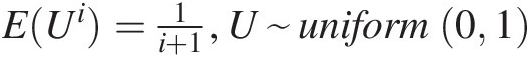
1. MECC construction only depends on the assigned constraints, that is, the Lagrange multipliers will not change in regard to different marginal distributions to be imposed. This is because (i) the marginals (i.e., CDFs) are uniformly distributed and EUi=1i+1,U~uniform01
 ; and (ii) the rank-based dependence measure does not depend on the marginal distributions.
2. E(Ui), E(Vi), i = 1, 2EUi,EVi,i=1,2 may be enough in regard to the marginal constraints to construct MECC (i.e., Equations (8.12a) and (8.12b)).
3. As shown in Example 8.2, the performance is not significantly improved by adding more constraints in dependence measure besides E(uv)Euv rather than making the optimization more complex.
4. In general, it is good enough to preserve the dependence measure through E(uv)Euv. E(uv)Euv directly corresponds to the rank-based Spearman correlation coefficient (ρsρs) (i.e., Equation (8.12c)). This is not unusual, since ρsρs is a popular nonparametric dependence measure used for parameter estimation besides Kendall’s tau (τ)τ).
5. The MECC constructed yields very similar performance, compared with the parametric copula with the same marginal distributions (e.g., the Gumbel–Hougaard copula applied in this chapter).
6. As with other parametric or nonparametric copulas, the marginal distributions and MECC can be investigated separately.
7. The overall advantage of MECC is that we obtain a unique Shannon entropy–based copula function with the given constraints. The parameters will not change with different marginal distribution candidates; however, parameters of parametric copulas do change if different marginal distribution candidates are used for parameter estimation. To some degree, the MECC minimizes the risk of improper choice of parametric copulas.
8. The MECC may be easily extended to a higher dimension with the use of a pairwise rank-based dependence structure.
