Abstract
In previous chapters, we have mainly discussed copula models for bivariate/multivariate random variables. Now we ask two other questions that usually arise in hydrology and water resources engineering. Can we use the stochastic approach to predict streamflow at a downstream location using streamflow at the upstream location? If streamflow is time dependent, then it cannot be considered as a random variable as is done in frequency analysis. Can we model the temporal dependence of an at-site streamflow sequence (e.g., monthly streamflow) more robustly than with the classical time series and Markov modeling approach (e.g., modeling the nonlinearity of time series freely)? This chapter attempts to address these questions and introduces how to model a time series with the use of copula approach.
9.1 General Concept of Time Series Modeling
In this section, we briefly introduce time series modeling. The reader may refer to Box et al. (2008) for a complete discussion. A time series (more specifically with even time intervals) may be stationary, nonstationary, or long-memory; linear or nonlinear. Following Box et al. (2008), a general form of a linear time series YtYt may be written as follows:
where YtYt is the time series; B is the backward operator; d is the differencing operator; d = 0d=0 for stationary; d is a positive integer (usually d = 1 or 2d=1or2) for nonstationary; d ∈ (0, 1)d∈01 for long memory time series; ϕ(B) = 1 − ϕ1B − ϕ2B2 − … − ϕpBpϕB=1−ϕ1B−ϕ2B2−···−ϕpBp is the autoregressive term; θ(B) = 1 + θ1B + θ2B2 + … + θqBqθB=1+θ1B+θ2B2+···+θqBq is the moving average term; and atat is the innovation (i.e., white noise and more specifically white Gaussian noise).
The classic time series model given in Equation (9.1) may be identified with the following procedures:
1. Graph the sample autocorrelation (ACF) and partial autocorrelation (PACF) function for time series {Xt : t = 1, …, n}Xt:t=1…n.
2. Identify the possible model order from sample ACF and PACF, if the visual evidences are observed:
i. If sample ACF falls into the 95% confidence bound quickly, then the time series XtXt may be considered stationary (shown in Figure 9.1(a)); otherwise, the time series is nonstationary or long memory (Figure 9.1(b)), and differencing is needed to convert a nonstationary time series into the stationary time series (Figure 9.1(c)).
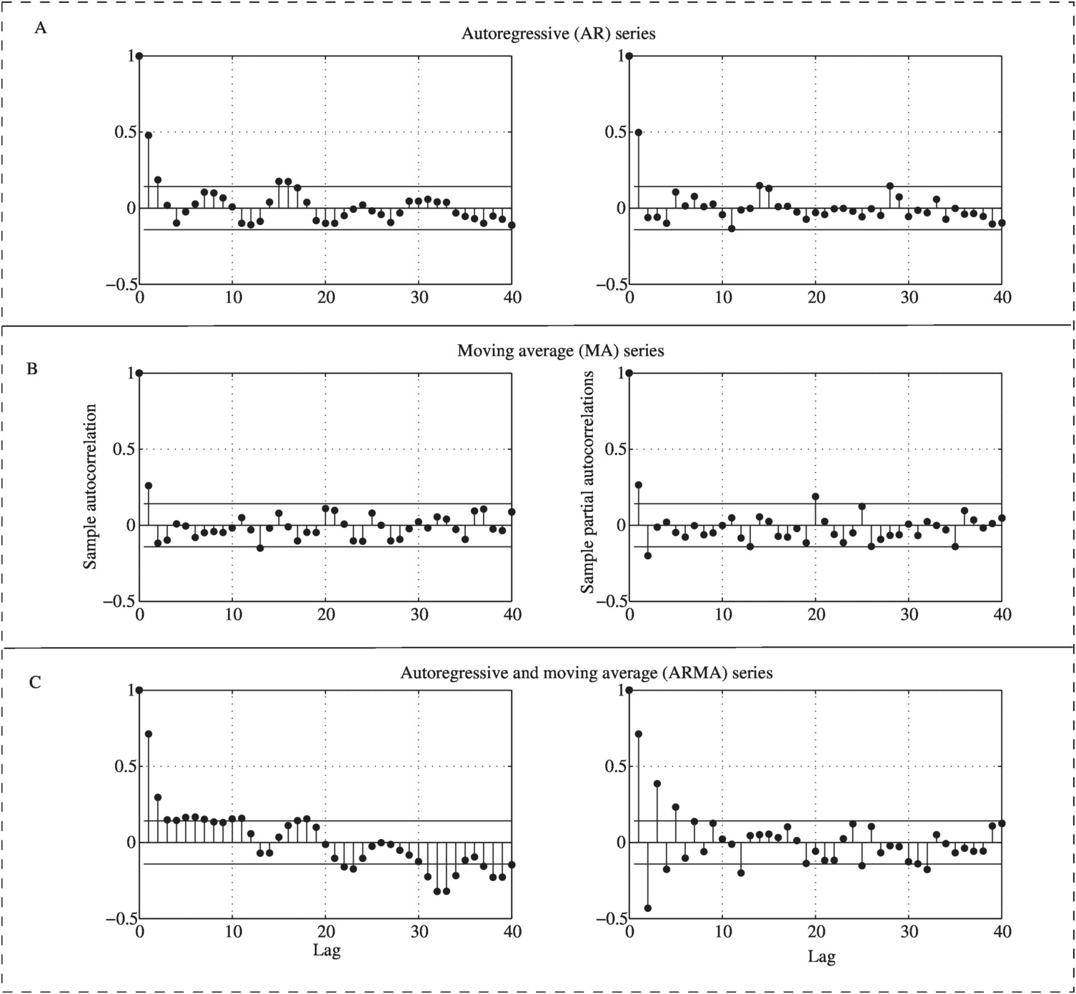
ii. With the stationary time series, the model order may then be estimated from the sample ACF and PACF as follows: (a) if the cutoff point in ACF with the PACF falls into the 95% confidence bound, we will have moving average (MA) time series model (Figure 9.2(a)); (b) if the cutoff point in PACF with the ACF falls into the 95% confidence bound, we will have autoregressive (AR) time series model (Figure 9.2(b)); and (c) if both ACF and PACF fall into the 95% confidence bound, we will have an autoregressive and moving average (ARMA) time series model (Figure 9.2(c)).
3. Estimate the model parameters for the stationary time series with the assumption of model residual: at~N0σa2
 .
.
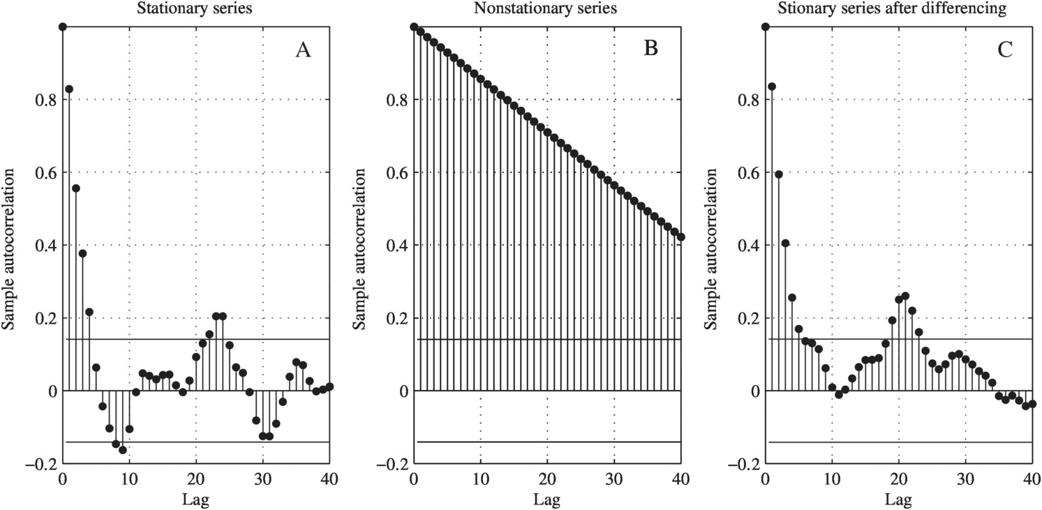
Figure 9.1 Sample autocorrelation function illustration plots.
With the preceding initial introduction, we will now further illustrate Equation (9.1) using streamflow as an example. It is supposed that the differencing order, d = 0, occurs most likely for a watershed before experiencing climate change and/or alteration by human activities; d = 1 occurs most likely for the watershed with these impacts; and d ∈ (0, 0.5)d∈00.5 occurs usually for reservoir operations. In other words, the original stationary streamflow series (or the stationary streamflow series after necessary differencing) at time t is dependent on the value at previous p times (i.e., it depends on the streamflow at t − 1, t − 2, …, t − pt−1,t−2,…,t−p). Constant c relates to the long-term average of the stationary series given in Equation (9.2b). θ(B) = 1 + θ1B + θ2B2 + … + θqBqθB=1+θ1B+θ2B2+…+θqBq represents the moving average term. Replacing wt = (1 − B)dYtwt=1−BdYt such that YtYt is now written as stationary time series after necessary differencing, Equation (9.1) may be rewritten as follows:
 (9.2)
(9.2)Taking the expectation of Equation (9.2), we have the following:
 (9.2a)
Substituting E(wt) = E(wt − i), i = 1, …, pEwt=Ewt−i,i=1,…,p, and E(at) = E(at − j) = 0Eat=Eat−j=0 for the stationary time series into Equation (9.2a), we have the following:
 (9.2b)
To further evaluate if differencing is necessary, two statistical tests can help make a reasonable and formal decision. The Kwiatkowski–Phillips–Schmidt–Shin (KPSS) test (1992) has the null hypothesis of time series being stationary, while the augmented Dickey–Fuller (ADF) test (Dickey and Fuller, 1979) has the null hypothesis of time series as a unit root process (or is simply called nonstationary). The KPSS and ADF tests are complementary to each other (Arya and Zhang, 2015) as follows:
i. Time series being stationary: acceptance by KPSS test while rejection by ADF test.
ii. Time series being nonstationary: rejection by KPSS test while acceptance by ADF test.
iii. Time series belonging to a long memory process: rejection by both KPSS and ADF tests. In this case, the Hurst coefficient (Hurst, 1951) is applied to evaluate the necessary fractional differencing order.
iv. Not enough evidence to decide whether the time series is stationary or nonstationary: acceptance by both KPSS and ADF tests.
Furthermore, if there exists heteroscedasticity (i.e., changing variance) in the time series such that the time series tends to have a large value following a large value and a small value following a small value as a simple illustration. Then, for the time series with heteroscedasticity, the model error of Equation (9.1) needs to be further revised using (Generalized) Autoregressive Conditional Heteroscedastic (G) (ARCH) models. A (G)ARCH model indicates a second-order dependent time series. In other words, the conditional variability depends on the past history of the time series. An ARCH model can be written as follows:
 (9.3)
(9.3)and a Generalized ARCH (Bollerslev, 1986) model can be written as follows:
 (9.4)
(9.4)In Equations (9.3) and (9.4), htht denotes the conditional variance (variability) of atat given at − 1, at − 2, …at−1,at−2,…; w0>0, wi ≥ 0, i = 1, …, s, qj ≥ 0, j = 1, …, rw0>0,wi≥0,i=1,…,s,qj≥0,j=1,…,r; wiwi denotes the coefficients of the ARCH effects (i.e., for the correlated squared model errors atat); and qiqi denotes the coefficients of the correlated conditional variance htht.
In addition, there exists a relation among conditional variance (ht)ht), innovation (i.e., model residual at)at) and standard white Guassian noise (et, et~N(0, 1))et,et~N01) as follows:
 (9.5)
(9.5)The parameters of the time series model may be estimated with the use of the maximum likelihood method.
Example 9.1 Fit an autoregressive time series model with order 1 (i.e., AR(1))Yt=c+ϕ1Yt−1+et,et~N0σe2 to annual streamflow data given in Table 9.1.

Plot the original time series and residual sequence. Is the residual sequence a white Gaussian noise?
Table 9.1. Annual streamflow data.
| Year | Flow (cfs) | Year | Flow (cfs) |
|---|---|---|---|
| 1960 | 517.9 | 1988 | 280.8 |
| 1961 | 367.8 | 1989 | 500.9 |
| 1962 | 252.2 | 1990 | 528.9 |
| 1963 | 258.6 | 1991 | 602.8 |
| 1964 | 281.3 | 1992 | 386 |
| 1965 | 308.4 | 1993 | 627.2 |
| 1966 | 317.3 | 1994 | 520 |
| 1967 | 372.4 | 1995 | 345.3 |
| 1968 | 349.1 | 1996 | 575 |
| 1969 | 504.3 | 1997 | 663.2 |
| 1970 | 330.9 | 1998 | 412.4 |
| 1971 | 413.3 | 1999 | 311 |
| 1972 | 461.7 | 2000 | 385.3 |
| 1973 | 567 | 2001 | 299.3 |
| 1974 | 500.6 | 2002 | 417.5 |
| 1975 | 654.9 | 2003 | 578.5 |
| 1976 | 550.3 | 2004 | 715.8 |
| 1977 | 401 | 2005 | 676.3 |
| 1978 | 593.8 | 2006 | 507 |
| 1979 | 508 | 2007 | 736 |
| 1980 | 543.5 | 2008 | 677.4 |
| 1981 | 442.3 | 2009 | 508.9 |
| 1982 | 477.3 | 2010 | 418.3 |
| 1983 | 473 | 2011 | 721.2 |
| 1984 | 548.3 | 2012 | 609 |
| 1985 | 467.7 | 2013 | 536.3 |
| 1986 | 539.3 | 2014 | 608.1 |
| 1987 | 431.7 | 2015 | 552.4 |
Solution: To fit AR(1) to the time series listed in Table 9.1, we can simply use the MATLAB function as follows:
1. Assign the TS as the time series listed in Table 9.1.
2. Set up the AR(1) model, where we need to fit using arima:
model=arima(1,0,0); % ARIMA (P, D, Q): P=1, AR term; D=0, stationary series; Q=0, MA term.
3. Apply the estimate function (through MLE):
[param,Var,LogL]=estimate(model,TS);
% param: estimated parameter for the model defined above.
% Var: variance-covariance matrix for the parameter estimated. Here, we have 3 parameters: constant-C, autoregressive parameter, and variance of model residual.
% LogL: the loglikelihood of the objective function after optimization.
Using the preceding functions, we get the results listed in Table 9.2.
Table 9.2. Parameter estimated for the AR(1) model.
| ARIMA (1,0,0) model (AR(1) model) | |||
|---|---|---|---|
| Conditional probability distribution: Gaussian | |||
| Parameter | Value | Standard error | T-statistics |
| Constant (cfs) | 255.13 | 71.80 | 3.55 |
| AR{1} | 0.475 | 0.15 | 3.18 |
| Variance (cfs2) | 12751.6 | 3141.41 | 4.06 |
| LogL = –434.18 | |||
The fitted AR(1) time series model is now written as follows:
4. Apply the infer function to compute the model residual sequence listed in Table 9.3:
res=infer(param,TS);
Table 9.3. Fitted model residual.
| Year | Residual (cfs) | Year | Residual (cfs) |
|---|---|---|---|
| 1960 | 24.90 | 1988 | –179.29 |
| 1961 | –133.22 | 1989 | 112.45 |
| 1962 | –177.55 | 1990 | 35.95 |
| 1963 | –116.27 | 1991 | 96.56 |
| 1964 | –96.61 | 1992 | –155.32 |
| 1965 | –80.29 | 1993 | 188.81 |
| 1966 | –84.25 | 1994 | –32.91 |
| 1967 | –33.38 | 1995 | –156.71 |
| 1968 | –82.84 | 1996 | 155.93 |
| 1969 | 83.43 | 1997 | 135.07 |
| 1970 | –163.66 | 1998 | –157.60 |
| 1971 | 1.07 | 1999 | –139.93 |
| 1972 | 10.34 | 2000 | –17.49 |
| 1973 | 92.67 | 2001 | –138.76 |
| 1974 | –23.73 | 2002 | 20.27 |
| 1975 | 162.10 | 2003 | 125.15 |
| 1976 | –15.76 | 2004 | 186.01 |
| 1977 | –115.40 | 2005 | 81.33 |
| 1978 | 148.28 | 2006 | –69.22 |
| 1979 | –29.05 | 2007 | 240.16 |
| 1980 | 47.18 | 2008 | 72.84 |
| 1981 | –70.87 | 2009 | –67.84 |
| 1982 | 12.18 | 2010 | –78.44 |
| 1983 | –8.74 | 2011 | 267.47 |
| 1984 | 68.60 | 2012 | 11.46 |
| 1985 | –47.75 | 2013 | –7.97 |
| 1986 | 62.12 | 2014 | 98.35 |
| 1987 | –79.48 | 2015 | 8.56 |
Figure 9.3 plots the original time series, fitted model residuals, and the histogram compared to the hypothesized white Gaussian noise. From the histogram plot, it seems that the hypothesized distribution may properly represent the distribution of the fitted model residuals. To formally assess whether the fitted model residuals are a white Gaussian noise, we apply the Kolmogorov–Smirnov (KS) test. The KS test evaluates the maximum distance of empirical and parametric CDFs. Its test statistic Dn can be written as follows:
 (9.7)
(9.7)The null hypothesis (H0) is that the fitted model residuals follow N0σe2,i.e.,N012751.6 . With this null hypothesis, we can either use the parametric bootstrap method or MATLAB function kstest directly. Here we will simply use the MATLAB function kstest. Table 9.4 lists the empirical and parametric CDFs for the fitted model residuals.

Figure 9.3 Original time series, fitted model residual plots, and histogram.
Table 9.4. Empirical and parametric CDFs of the fitted model residuals.
| Residual | Parametric CDF | Empirical CDF | Residual | Parametric CDF | Empirical CDF |
|---|---|---|---|---|---|
| 24.90 | 0.59 | 0.63 | –179.29 | 0.06 | 0.02 |
| –133.22 | 0.12 | 0.16 | 112.45 | 0.84 | 0.82 |
| –177.55 | 0.06 | 0.04 | 35.95 | 0.62 | 0.65 |
| –116.27 | 0.15 | 0.18 | 96.56 | 0.80 | 0.79 |
| –96.61 | 0.20 | 0.21 | –155.32 | 0.08 | 0.11 |
| –80.29 | 0.24 | 0.26 | 188.81 | 0.95 | 0.95 |
| –84.25 | 0.23 | 0.23 | –32.91 | 0.39 | 0.40 |
| –33.38 | 0.38 | 0.39 | –156.71 | 0.08 | 0.09 |
| –82.84 | 0.23 | 0.25 | 155.93 | 0.92 | 0.89 |
| 83.43 | 0.77 | 0.75 | 135.07 | 0.88 | 0.86 |
| –163.66 | 0.07 | 0.05 | –157.60 | 0.08 | 0.07 |
| 1.07 | 0.50 | 0.53 | –139.93 | 0.11 | 0.12 |
| 10.34 | 0.54 | 0.56 | –17.49 | 0.44 | 0.46 |
| 92.67 | 0.79 | 0.77 | –138.76 | 0.11 | 0.14 |
| –23.73 | 0.42 | 0.44 | 20.27 | 0.57 | 0.61 |
| 162.10 | 0.92 | 0.91 | 125.15 | 0.87 | 0.84 |
| –15.76 | 0.44 | 0.47 | 186.01 | 0.95 | 0.93 |
| –115.40 | 0.15 | 0.19 | 81.33 | 0.76 | 0.74 |
| 148.28 | 0.91 | 0.88 | –69.22 | 0.27 | 0.33 |
| –29.05 | 0.40 | 0.42 | 240.16 | 0.98 | 0.96 |
| 47.18 | 0.66 | 0.67 | 72.84 | 0.74 | 0.72 |
| –70.87 | 0.27 | 0.32 | –67.84 | 0.27 | 0.35 |
| 12.18 | 0.54 | 0.60 | –78.44 | 0.24 | 0.30 |
| –8.74 | 0.47 | 0.49 | 267.47 | 0.99 | 0.98 |
| 68.60 | 0.73 | 0.70 | 11.46 | 0.54 | 0.58 |
| –47.75 | 0.34 | 0.37 | –7.97 | 0.47 | 0.51 |
| 62.12 | 0.71 | 0.68 | 98.35 | 0.81 | 0.81 |
| –79.48 | 0.24 | 0.28 | 8.56 | 0.53 | 0.54 |
Applying kstest as follows
[H,Pvalue,stat]=kstest(res,[res,normcdf(res,0,param.Variance^0.5)],0.05)
we have H = 0, Pvalue = 0.803, and test statistic = 0.083. With null hypothesis being accepted and Pvalue > 0.05, we show that the fitted model residual is a white Gaussian noise.
9.2 Spatially Dependent Bivariate or Multivariate Time Series
In stock exchanges, the stock values among major exchanges (e.g., London, Hong Kong, New York, Tokyo) always impact one another. In other words, these major exchanges have a tendency to follow each other. In the field of hydrology and water resources engineering, there also exists a similar tendency (or spatial dependence). For example, streamflow (or flood) at a downstream location is generally positively dependent on that at the upstream location. In this section, we will show how to evaluate spatially dependent time series.
As discussed in the previous chapters, copulas are applied to bivariate/multivariate independent random variables. Thus, to employ the copula theory for a bivariate (multivariate) time-dependent sequence (e.g., spatial dependence of bivariate/multivariate time series), we need to investigate each individual time series first and fit the time series with proper models (e.g., the equations in Section 9.1). Three steps are needed for bivariate/multivariate time series analysis using copulas:
1. Investigate each univariate time series separately, including the assessment of stationarity, time series model identification, and estimation of model parameters;
2. Compute model residuals from the fitted univariate time series model.
3. Apply copulas to the model residuals obtained from step 2.
In what follows, we will use a simple example to illustrate how to model a bivariate time series.
Example 9.2 Perform a dependence study using the daily time series data given in Table 9.5.
Table 9.5. Bivariate time series.
| TS1 | TS2 | TS1 | TS2 | ||
|---|---|---|---|---|---|
| 1 | 60.25 | 476.35 | 26 | 45.24 | 475.13 |
| 2 | 55.87 | 475.48 | 27 | 11.28 | 475.01 |
| 3 | 76.18 | 476.02 | 28 | 30.96 | 475.44 |
| 4 | 74.84 | 476.75 | 29 | 78.03 | 475.49 |
| 5 | 84.79 | 476.89 | 30 | 97.69 | 475.91 |
| 6 | 68.39 | 477.27 | 31 | 90.31 | 476.52 |
| 7 | 73.14 | 477.51 | 32 | 60.44 | 475.51 |
| 8 | 63.01 | 476.50 | 33 | 52.28 | 474.24 |
| 9 | 63.28 | 475.87 | 34 | 35.00 | 473.57 |
| 10 | 80.17 | 475.74 | 35 | 38.98 | 473.33 |
| 11 | 72.42 | 475.29 | 36 | 49.74 | 473.42 |
| 12 | 57.82 | 476.75 | 37 | 75.43 | 473.87 |
| 13 | 86.49 | 476.60 | 38 | 81.49 | 471.65 |
| 14 | 99.88 | 475.69 | 39 | 56.48 | 470.84 |
| 15 | 75.34 | 474.94 | 40 | 51.48 | 472.87 |
| 16 | 66.07 | 473.83 | 41 | 50.26 | 473.17 |
| 17 | 56.61 | 473.63 | 42 | 52.20 | 474.16 |
| 18 | 69.76 | 473.84 | 43 | 76.67 | 475.32 |
| 19 | 94.75 | 475.58 | 44 | 83.07 | 475.63 |
| 20 | 62.69 | 476.17 | 45 | 79.80 | 475.90 |
| 21 | 64.71 | 475.11 | 46 | 81.26 | 474.64 |
| 22 | 88.54 | 476.29 | 47 | 73.69 | 474.19 |
| 23 | 84.75 | 478.09 | 48 | 72.70 | 476.01 |
| 24 | 94.86 | 478.04 | 49 | 77.68 | 476.85 |
| 25 | 81.05 | 476.20 | 50 | 89.06 | 476.79 |
Solution: Applying the procedure similar to Example 9.1, the time series TS1 and TS2 are fitted with ARIMA (1,0,1) (i.e., ARMA(1,1)) and ARIMA(2,0,0) (i.e., AR(2)), respectively. The fitted parameters for the time series are given in Table 9.6. Figure 9.4 plots the original time series and empirical frequencies (histogram) for the model residuals.
Table 9.6. Fitted time series model and parameter estimated.
| TS1-ARIMA(1,0,1) model: | |||
| conditional probability distribution: Gaussian | |||
| Parameter | Value | Standard error | T statistics |
| Constant | 55.24 | 13.18 | 4.19 |
| AR{1} | 0.21 | 0.19 | 1.09 |
| MA{1} | 0.66 | 0.15 | 4.34 |
| Variance | 185.21 | 42.53 | 4.36 |
| TS2-ARIMA(2,0,0) model: | |||
| conditional probability distribution: Gaussian | |||
| Parameter | Value | Standard error | T statistics |
| Constant | 125.18 | 38.95 | 3.16 |
| AR{1} | 1.1 | 0.15 | 7.15 |
| AR{2} | –0.36 | 0.16 | –2.3 |
| Variance | 0.7 | 0.12 | 5.63 |

Figure 9.4 Plots of original time series and histograms of the fitted model residuals.
The acceptance by the KS test for the fitted model residuals indicates that the model residuals belong to the white noise.
We can write the residuals as a function of time series:
 (9.8a)
 (9.8b)
Now, we may apply copula to restTS1,restTS2 that are considered as independent random variables. Figure 9.5 shows the scatter plot of the random variables.

Figure 9.5 Scatter plot of the fitted model residuals: restT1 and restT2
 .
.
From Figure 9.5, it is seen the fitted model residuals are positively correlated. Using Equations (3.70) and (3.73), the empirical rank-based correlation coefficients, Spearman’s ρ, and Kendall’s τ are computed as ρn≈0.28, τn≈0.16ρn≈0.28,τn≈0.16. To this end, we apply the Archimedean copulas (i.e., Gumbel–Hougaard, Clayton, and Frank copulas presented in Chapter 4) and meta-elliptical copulas (i.e., the Gaussian and Student t copulas presented in Chapter 7). Similar to the discussion in the previous chapters, we apply the pseudo (i.e., semiparametric) and two-stage maximum likelihood methods for parameter estimation. Table 9.7 lists the empirical and parametric CDFs of the fitted model residuals. Table 9.8 lists the parameters and corresponding estimated likelihood values. The likelihood values in Table 9.8 suggest that the Frank copula attains the best overall performance, followed by Gaussian copula. Figure 9.6 compares the CDF of the model residuals to the simulated random variates from the fitted parametric copulas. Figure 9.7 compares the model residuals to that computed from the two-stage estimation. Comparison indicates a similar performance between the Frank and Gaussian copulas.
Table 9.7. Fitted model residuals, empirical and parametric CDFs computed.
restT1 | restT2 | Empirical CDF | Parametric CDF | ||
|---|---|---|---|---|---|
restT1 | restT2 | restT1 | restT2 | ||
| –9.03 | 0.13 | 0.25 | 0.59 | 0.25 | 0.56 |
| –5.91 | –0.59 | 0.31 | 0.20 | 0.33 | 0.24 |
| 13.25 | 0.89 | 0.78 | 0.86 | 0.83 | 0.86 |
| –4.93 | 0.72 | 0.39 | 0.82 | 0.36 | 0.80 |
| 17.28 | 0.24 | 0.92 | 0.67 | 0.90 | 0.61 |
| –15.82 | 0.73 | 0.14 | 0.84 | 0.12 | 0.81 |
| 14.15 | 0.60 | 0.80 | 0.80 | 0.85 | 0.76 |
| –16.72 | –0.53 | 0.12 | 0.24 | 0.11 | 0.26 |
| 5.99 | 0.03 | 0.67 | 0.57 | 0.67 | 0.51 |
| 7.86 | 0.23 | 0.69 | 0.65 | 0.72 | 0.61 |
| –4.62 | –0.29 | 0.41 | 0.35 | 0.37 | 0.36 |
| –9.39 | 1.60 | 0.24 | 0.94 | 0.24 | 0.97 |
| 25.46 | –0.31 | 0.98 | 0.33 | 0.97 | 0.36 |
| 9.94 | –0.53 | 0.71 | 0.22 | 0.77 | 0.26 |
| –7.15 | –0.33 | 0.27 | 0.31 | 0.30 | 0.35 |
| –0.08 | –0.94 | 0.51 | 0.14 | 0.50 | 0.13 |
| –12.28 | –0.19 | 0.18 | 0.37 | 0.18 | 0.41 |
| 10.88 | –0.16 | 0.73 | 0.43 | 0.79 | 0.42 |
| 17.88 | 1.28 | 0.94 | 0.90 | 0.91 | 0.94 |
| –23.98 | 0.02 | 0.06 | 0.53 | 0.04 | 0.51 |
| 12.28 | –1.06 | 0.76 | 0.10 | 0.82 | 0.10 |
| 11.79 | 1.51 | 0.75 | 0.92 | 0.81 | 0.96 |
| 3.38 | 1.62 | 0.55 | 0.96 | 0.60 | 0.97 |
| 19.83 | 0.01 | 0.96 | 0.51 | 0.93 | 0.50 |
| –6.93 | –1.12 | 0.29 | 0.06 | 0.31 | 0.09 |
| –22.24 | –0.19 | 0.08 | 0.39 | 0.05 | 0.41 |
| –38.68 | 0.22 | 0.02 | 0.61 | 0.00 | 0.60 |
| –1.12 | 0.38 | 0.47 | 0.73 | 0.47 | 0.68 |
| 17.11 | –0.08 | 0.90 | 0.47 | 0.90 | 0.46 |
| 14.99 | 0.45 | 0.86 | 0.75 | 0.86 | 0.70 |
| 4.93 | 0.60 | 0.59 | 0.78 | 0.64 | 0.76 |
| –16.78 | –0.93 | 0.10 | 0.16 | 0.11 | 0.13 |
| –4.43 | –0.85 | 0.43 | 0.18 | 0.37 | 0.15 |
| –28.16 | –0.51 | 0.04 | 0.25 | 0.02 | 0.27 |
| –4.96 | –0.45 | 0.37 | 0.27 | 0.36 | 0.30 |
| –10.31 | –0.35 | 0.22 | 0.29 | 0.22 | 0.34 |
| 16.67 | –0.08 | 0.88 | 0.49 | 0.89 | 0.46 |
| –0.37 | –2.76 | 0.49 | 0.02 | 0.49 | 0.00 |
| –15.41 | –0.97 | 0.16 | 0.12 | 0.13 | 0.12 |
| –5.32 | 1.16 | 0.35 | 0.88 | 0.35 | 0.92 |
| –12.14 | –1.08 | 0.20 | 0.08 | 0.19 | 0.10 |
| –5.46 | 0.32 | 0.33 | 0.69 | 0.34 | 0.65 |
| 14.21 | 0.49 | 0.82 | 0.76 | 0.85 | 0.72 |
| 2.57 | –0.11 | 0.53 | 0.45 | 0.57 | 0.45 |
| 5.65 | 0.23 | 0.63 | 0.63 | 0.66 | 0.61 |
| 5.76 | –1.21 | 0.65 | 0.04 | 0.66 | 0.07 |
| –2.19 | -0.18 | 0.45 | 0.41 | 0.44 | 0.42 |
| 3.63 | 1.68 | 0.57 | 0.98 | 0.61 | 0.98 |
| 4.98 | 0.36 | 0.61 | 0.71 | 0.64 | 0.67 |
| 14.43 | 0.03 | 0.84 | 0.55 | 0.86 | 0.51 |
Table 9.8. Estimated copula parameters and estimated log-likelihood values.
| Copula | Pseudo | MLE | Semiparametric | MLE |
|---|---|---|---|---|
| Gumbel–Hougaard | 1.15 | 0.75 | 1.13 | 0.61 |
| Clayton | 0.31 | 0.88 | 0.08 | 0.15 |
| Frank | 1.63 | 1.79 | 1.56 | 1.69 |
| Gaussian | 0.26 | 1.30 | 0.20 | 0.99 |
| Student t | [0.26, 1.38 × 10⁷]0.261.38×107 | 1.30 | [0.20, 1.38 × 10⁷]0.201.38×107 | 0.99 |

Figure 9.6 Comparison of simulated random variates to pseudo-observations and fitted parametric marginals.

Figure 9.7 Comparison of fitted model residuals to those computed from copula with parameter estimated using two-stage MLE.
From this example, we also note that the rank-based correlation coefficient of the model residuals may be different from that of the original time series. In this example, we have τn≈0.16τn≈0.16 for the model residuals, while τn≈0.35τn≈0.35 for the original time series. The reduction of the degree of association for the model residuals may be due to the autoregressive component of time series modeling.
From Equation (9.8), we can also reconstruct the time series with the use of random variates from the simulated copula. Here, we will again use copulas with two-stage MLE as an example. Additionally, we will use the last two values of the time series (i.e., Table 9.5) as initial estimates. Figure 9.8 plots the reconstructed time series, which shows that the reconstructed time series reasonably follows the same pattern as does the original time series.

Figure 9.8 Reconstructed time series using the copula estimated with two-stage MLE.
Now, we have explained how to study the spatial dependence for the sequence with time dependence. In the previous example, we studied time-dependent sequences and spatial dependence of the sequences separately. We first built the time series (i.e., the autoregressive and moving average) model for each univariate time-dependent sequence. Then, we built the copula model on the residual (also called innovation) of the time series model, since the residuals are now random variables.
Copula modeling can also be applied to study the serial dependence of univariate time series, in addition to studying the previously discussed bivariate/multivariate spatial-temporal dependent time series (i.e., spatial dependence for the time-dependent sequence). In the following section, we will introduce how to model the serial dependence of univariate time series.
9.3 Copula Modeling for Univariate Time Series with Serial Dependence: General Discussion
Darsow, et al. (1992) introduced the condition (i.e., equivalent to Chapman–Kolmogorov equations) for a copula-based time series to be a Markov process. Joe (1997) introduced a class of parametric stationary Markov models based on parametric copulas and parametric marginal distributions. Similar to the copula application in bivariate or multivariate frequency analysis discussed previously, a copula-based time series model also allows one to consider serial dependence and marginal behavior of the time series investigated separately.
Following Joe (1997) and Chen and Fan (2006), copulas can be applied to the stationary time series of (i) Markov chain models (both discrete and continuous, including autoregressive models); (ii) K-dependent time series models (i.e., moving average models with order k); (iii) convolution-closed infinitely divisible univariate marginal models. For stationary time series {Zt : t = 1, 2, …}Zt:t=12….
Let {et}et be i.i.d. random variables that are independent of {Zt − 1, Zt − 2…}Zt−1Zt−2… (i.e., the innovation of the time series {Zt : t = 1, 2, …Zt:t=1,2,…}). We may express the preceding three cases by using one of the following models (Joe, 1997).
Markov Chain models:
➣ Kth-order autoregressive model:
where α1, α2, …, αKα1,α2,…,αK are the scalars.
Zt = α1Zt − 1 + αtZt − 2 + … + αKZt − K + etZt=α1Zt−1+αtZt−2+···+αKZt−K+et(9.9)
➣ Kth-order Markov chain:
where gg is a real-valued function.
Zt = g(Zt − 1, Zt − 2, …, Zt − k, et)Zt=gZt−1Zt−2…Zt−ket(9.10)
➣ First-order convolution-closed infinitely divisional univariate margin model:
where StSt is an independent realization of the stochastic operator.
Zt = St(Zt − 1) + ϵtZt=StZt−1+et(9.11)
K-dependent time series models:
➣ Kth-order Moving Average model:
where β1, β2, …, βKβ1,β2,…,βK are the scalars.
Zt = et + β1et − 1 + β2et − 2 + … + βKet − KZt=et+β1et−1+β2et−2+···+βKet−K(9.12)
➣ K-dependent model:
where hh is a real-valued function.
Zt = h(et, et − 1, …, et − K)Zt=hetet−1…et−K(9.13)
➣ One-dependent convolution-closed infinitely divisible univariate marginal model:
Zt = et + St(et − 1)Zt=et+Stet−1(9.14)
where StSt is the independent realization of the stochastic operator.
Now, with the classified models given in Equations (9.10)–(9.14), we will focus on the continuous Markov chain (also called Markov process) models for the rest of the chapter. We will introduce the simple first-order Markov models first, followed by the Kth-order Markov models.
9.4 First-Order Copula-Based Markov Model
9.4.1 General Concept of the First-Order Copula-Based Continuous Markov Model
For continuous time series {Zt : t = 1, 2, …}Zt:t=12… modeled with the first-order Markov process, its transition probability can be expressed as follows:
Equation (9.15) means that the probabilistic behavior of the time series {Zt}Zt is fully governed by the joint distribution of {Zt, Zt − 1}ZtZt−1. We can apply copula modeling as a robust and powerful representation of Equation (9.15) as follows:
 (9.16a)
and the conditional density of ZtZt given Zt − 1Zt−1 can be expressed using copula as follows:
where CC and cc represent the copula and its density function of (zt, zt − 1(zt,zt−1), and FF and ff represent the marginal distribution and the density function of ztzt, respectively
9.4.2 Parameter Estimation of the First-Order Copula-Based Continuous Markov Model
Chen and Fan (2006) proposed an estimation method similar to the semiparametric maximum likelihood estimation method discussed in the previous chapters. Following Chen and Fan (2006) and Equations (9.16a) and (9.16b), we see the time series is fully determined by the true unknown marginal distribution F∗F∗ and a copula function with parameter α∗α∗ (or simply written as (F∗, α∗)F∗α∗). Here we again note the advantage of investigating the marginal distribution and copula separately.
To evaluate the copula parameter, we may first apply the empirical marginal to time series {Zt}Zt with the Weibull plotting-position formula in the same fashion as Equation (3.103):
 (9.17)
where: mm is the length of time series (or simply called the sample size).
Replacing Equation (9.17) with the true unknown marginal and its density function, and true copula density function, the log-likelihood function for the first-order Markov model can be expressed as follows:
 (9.18a)
Equation (9.18a) can be simplified using the empirical distribution FnFn as follows:
 (9.18b)
Equation (9.18b) is in the same form as Equation (3.104).
9.4.3 Simulation (Realizations) of the Time Series from the First-Order Copula-Based Markov Process
The univariate time series from the first-order copula-based Markov process can be simulated with a similar approach discussed in Section 3.7. With little modification, the simulation procedure is presented as follows:
i. Generate i.i.d. uniformly distributed random variables U = {ui : i = 1, 2, 3, …, N}U=ui:i=123…N.
ii. Set y1 = u1y1=u1.
iii. Set u2=Cy2y1=Cy2u1=∂Cy2u1∂u1⇒y2=h−1u2y1α
 , in which the hh function is defined as the conditional copula.
iv. Continue until we obtain yN = h−1(un, yn − 1; α)yN=h−1unyn−1α.

It should be noted that {y1, y2, …, yn}y1y2…yn simulated from steps i to iv are the time series in the frequency domain (i.e., marginals), and we will need to perform the one-to-one transformation to obtain the corresponding time series simulated in the real domain (e.g., through parametric distribution, empirical distribution, or kernel density based on the observed time series).
9.4.4 Forecast and Quantile Estimation of the First-Order Markov Process
As in economics and finance, it is our interest to forecast the future behavior of the time series, or in other words median forecast and conditional quantile estimation. For given quantile, the conditional quantile estimation may also be called value-at-risk (VaR). From the transitional probability of the first-order Markov process (i.e., Equation (9.16a)), we have the median forecast expressed as follows:
 (9.19a)
Again, replacing the unknown true marginal distribution by its empirical distribution, and the true copula parameter by its estimated parameter (α̂ ) from Equation (9.18b), Equation (9.19a) can be rewritten as follows:
 (9.19b)
Equation (9.19b) implies that the conditional probability (i.e., conditional copula) of Zt ∣ Zt − 1Zt∣Zt−1 equals 0.5 (also called 50% conditional quantile) as follows:
 (9.20a)
From Equation (9.20a), we can further forecast the behavior of ztzt as follows:
 (9.20b)
Similarly, Equations (9.20a) and (9.20b) can be easily reformulated for the estimation of any given conditional quantile q as follows:
 (9.21)
Example 9.3 Rework Example 9.1 using the Gumbel–Hougaard and Gaussian copula-based first-order Markov model. Also, compare the one-step ahead forecast (i.e., forecasting the annual flow for water year 2016) with both the classic AR(1) model and copula-based first-order Markov model.
Solution: In Example 9.1, we applied the AR(1) model to investigate the behavior and annual flow listed in Table 9.1. From Example 9.1 we conclude that statistically, we can apply AR(1) model to the annual flow under the assumption that annual flow shows a linear temporal dependence; however, in reality the dependence is usually nonlinear. Without imposing more complex (G)ARCH model, the copula-based Markov model is an excellent alternative approach to solve this issue. In addition, the Gaussian process assumption is also relaxed when applying the copula-based Markov model.
In this example, we will use semiparametric estimation such that the empirical distribution is applied for the marginals. The following steps are needed to model the temporal dependence with copulas:
1. With Equation (9.17), the Weibull plotting position formula and kernel density function are employed to compute the empirical marginal distribution (Table 9.9). It is worth noting that the marginal estimated nonparametrically will not change the structure of the time series dataset, as shown in Figure 9.9 (through the sample autocorrelation function plot).
2. Estimate the copula parameter for the first-order Markov model using Equation (9.17b).
3. Estimate the copula parameter for the first-order Markov model using Equation (9.17b).
Table 9.9. Empirical marginals using the Weibull plotting position formula and kernel density function.
| (1) | (2) | (3) | (4) | (1) | (2) | (3) | (4) |
|---|---|---|---|---|---|---|---|
| 1960 | 517.9 | 0.58 | 0.58 | 1988 | 280.8 | 0.05 | 0.08 |
| 1961 | 367.8 | 0.21 | 0.23 | 1989 | 500.9 | 0.49 | 0.53 |
| 1962 | 252.2 | 0.02 | 0.05 | 1990 | 528.9 | 0.61 | 0.61 |
| 1963 | 258.6 | 0.04 | 0.06 | 1991 | 602.8 | 0.81 | 0.79 |
| 1964 | 281.3 | 0.07 | 0.08 | 1992 | 386 | 0.26 | 0.26 |
| 1965 | 308.4 | 0.11 | 0.12 | 1993 | 627.2 | 0.86 | 0.84 |
| 1966 | 317.3 | 0.14 | 0.13 | 1994 | 520 | 0.60 | 0.59 |
| 1967 | 372.4 | 0.23 | 0.23 | 1995 | 345.3 | 0.18 | 0.18 |
| 1968 | 349.1 | 0.19 | 0.19 | 1996 | 575 | 0.75 | 0.73 |
| 1969 | 504.3 | 0.51 | 0.54 | 1997 | 663.2 | 0.89 | 0.89 |
| 1970 | 330.9 | 0.16 | 0.16 | 1998 | 412.4 | 0.30 | 0.32 |
| 1971 | 413.3 | 0.32 | 0.32 | 1999 | 311 | 0.12 | 0.12 |
| 1972 | 461.7 | 0.40 | 0.43 | 2000 | 385.3 | 0.25 | 0.26 |
| 1973 | 567 | 0.74 | 0.71 | 2001 | 299.3 | 0.09 | 0.11 |
| 1974 | 500.6 | 0.47 | 0.53 | 2002 | 417.5 | 0.33 | 0.33 |
| 1975 | 654.9 | 0.88 | 0.88 | 2003 | 578.5 | 0.77 | 0.74 |
| 1976 | 550.3 | 0.70 | 0.67 | 2004 | 715.8 | 0.95 | 0.95 |
| 1977 | 401 | 0.28 | 0.29 | 2005 | 676.3 | 0.91 | 0.91 |
| 1978 | 593.8 | 0.79 | 0.77 | 2006 | 507 | 0.53 | 0.55 |
| 1979 | 508 | 0.54 | 0.55 | 2007 | 736 | 0.98 | 0.96 |
| 1980 | 543.5 | 0.67 | 0.65 | 2008 | 677.4 | 0.93 | 0.91 |
| 1981 | 442.3 | 0.39 | 0.39 | 2009 | 508.9 | 0.56 | 0.56 |
| 1982 | 477.3 | 0.46 | 0.47 | 2010 | 418.3 | 0.35 | 0.33 |
| 1983 | 473 | 0.44 | 0.46 | 2011 | 721.2 | 0.96 | 0.95 |
| 1984 | 548.3 | 0.68 | 0.66 | 2012 | 609 | 0.84 | 0.80 |
| 1985 | 467.7 | 0.42 | 0.45 | 2013 | 536.3 | 0.63 | 0.63 |
| 1986 | 539.3 | 0.65 | 0.64 | 2014 | 608.1 | 0.82 | 0.80 |
| 1987 | 431.7 | 0.37 | 0.36 | 2015 | 552.4 | 0.72 | 0.67 |
Note: (1): year; (2): annual flow (cfs); (3): empirical CDF; (4): CDF computed through kernel density.

Figure 9.9 Sample autocorrelation function plots for original Flow series, rank-based and kernel density based marginals.
As discussed in the previous chapters, we can first estimate the rank-based Kendall’s tau for lag-1 temporal dependence. We computed τ≈0.31τ≈0.31. As the autoregressive coefficient estimated in Example 9.1 (φ≈0.47φ≈0.47), the annual flow at the current time tt is positively dependent on that at the previous time of t − 1t−1. Using computed sample τ≈0.31τ≈0.31, we obtain the initial parameter estimate:


Now maximizing Equation (9.18b) for the log-likelihood functions of Gumbel–Hougaard and meta-Gaussian copulas, we have θGH = 1.38; θGAU = 0.51θGH=1.38;θGAU=0.51.
Comparing to the parameter estimated from the AR(1) model and that estimated from meta-Gaussian copula-based first-order Markov model, there is minimal difference in regard to the parameter estimated. To further compare AR(1) model and copula-based first-order Markov model, we simulate the time series with 100 realizations. We directly simulate the realizations in the real domain for the AR(1) model (with the parameters estimated in Example 9.1). For the copula-based first-order Markov process, we first simulate the marginals, and then we perform the inverse transformation with the kernel density function approach. Figure 9.10 plots the realizations from all three approaches.

One-step ahead forecast with the AR(1) model: From Equation (9.6), the corresponding one-step ahead forecast is written using the difference equation as [Zt + 1] = 255.132 + 0.475[Zt] + [ϵt + 1]Zt+1=255.132+0.475Zt+ϵt+1.
Substituting [ϵt + 1] = 0ϵt+1=0 and z2015 = 552.4 cfsz2015=552.4cfs into the forecast equation, we have the following:
[z2016] = 255.132 + 0.475(552.4) = 517.52 cfsz2016=255.132+0.475552.4=517.52cfs.
One-step ahead forecast from copula-based first-order Markov models: First, we can rewrite Equation (9.20b) in a similar fashion as the preceding AR(1) forecast equation:
 (9.22)
In Equation (9.22) FnFn represents the marginal estimated nonparametrically through the kernel density function.
i. Gumbel–Hougaard copula: Substituting α̂=1.38
 and Fn(z2015) = 0.67Fnz2015=0.67 into Equation (9.22) for Gumbel–Hougaard copula, we obtain the estimated marginal for 2016 and the corresponding forecasted annual flow as follows:
[Fn(z2016)]GH = 0.56, and [z2016]GH = 509.36 cfsFnz2016GH=0.56,andz2016GH=509.36cfs
ii. Meta-Gaussian copula: Substituting α̂=0.514
 and Fn(z2015) = 0.67Fnz2015=0.67 into Equation (8.22) for the meta-Gaussian copula, we obtain the estimated marginal for 2016 and the corresponding forecasted annual flow as follows:
[Fn(z2016)]GAU = 0.591, and [z2016]GAU = 521.62 cfsFnz2016GAU=0.591,andz2016GAU=521.62cfs


Comparing the one-step ahead forecast with the AR(1) and meta-Gaussian copula-based first-order Markov model, it is seen that the relative difference of forecast results is less than 1% with the meta-Gaussian copula reaching a slightly better forecasting result.
9.5 Kth-Order Copula-Based Markov Models (K ≥ 2K≥2)
Similar to the discussion in Section 9.4; the continuous time series {Zt : t = 1, 2, …}Zt:t=12…, modeled by the Kth-order Markov process, is fully governed by the joint distribution of {Zt, Zt − 1, …, Zt − k}ZtZt−1…Zt−k. The transition probability for the first-order Markov process (i.e., Equation (9.15)) can be rewritten as follows:
Similar to the application of bivariate copula to study the first-order Markov models, the serial dependence of Kth order copula-based Markov process may be fully assessed using (K+1)-dimensional copulas.
9.5.1 Building Copula Structure for Kth-Order Markov Models
Given the property of serial dependence for a higher-order Markov process, we need to construct a D-vine copula for the modeling purpose.
We will use a third-order Markov process as an example (Figure 9.11 similar to Figure 5.11).

Figure 9.11 D-vine copula for a third-order Markov process.
To comply with the properties of the Markov process, Figure 9.11 shows the following:
a. The same as the first-order Markov model, zt, zt − 1, zt − 2, and zt − 3zt,zt−1,zt−2,andzt−3 have the same marginal distribution.
b. T1 directly represents the lag-1 serial dependence, i.e., the same copula applies to {zt, zt − 1}, {zt − 1, zt − 2}, {zt − 2, zt − 3}ztzt−1,zt−1zt−2,zt−2zt−3, i.e., Ct, t − 1 ≡ Ct − 1, t − 2 ≡ Ct − 2, t − 3Ct,t−1≡Ct−1,t−2≡Ct−2,t−3.
c. For the lag-2 serial dependence, we also have the same copula applying to {zt, zt − 1, zt − 2}, {zt − 1, zt − 2, zt − 3}ztzt−1zt−2,zt−1zt−2zt−3, i.e., Ct, t − 1, t − 2 ≡ Ct − 1, t − 2, t − 3Ct,t−1,t−2≡Ct−1,t−2,t−3.
d. The copulas in b and c are differentiable.
With the same philosophy, we can model the given Kth-order Markov process using copulas.
9.5.2 Order Identification for the Markov Process
We have explained how to build a copula structure for higher-order Markov process. Here we further explain how to identify the order of Markov process for the time series with the following procedure:
i. Study the lag-1 dependence by evaluating the dependence of {Fzt, Fzt − 1}FztFzt−1. If FztFzt and Fzt − 1Fzt−1 are stochastically independent, we say there is no lag-1 dependence (or say ztzt and zt − 1zt−1 are independent).
ii. If step i indicates the lag-1 dependence being statistically significant, we evaluate the dependence of {Fzt, Fzt − 2}FztFzt−2 for lag-2 dependence of ztzt and zt − 2zt−2 through the evaluation of Ft ∣ t − 1(zt| zt − 1)Ft∣t−1ztzt−1 and Ft − 2 ∣ t − 1(zt − 2| zt − 1)Ft−2∣t−1zt−2zt−1 (i.e., the copula form of Ct ∣ t − 1(F(zt)| F(zt − 1))Ct∣t−1FztFzt−1 and Ct − 2 ∣ t − 1(F(zt − 2)| F(zt − 1))Ct−2∣t−1Fzt−2Fzt−1.
iii. We move sequentially to higher orders until we identify that Ft ∣ t − 1, …, t − kFt∣t−1,…,t−k and Ft − (k + 1) ∣ t − 1, …, t − kFt−k+1∣t−1,…,t−k (i.e., Ct ∣ t − 1, …, t − kCt∣t−1,…,t−k and Ct − k − 1 ∣ t − 1, …, t − kCt−k−1∣t−1,…,t−k) are stochastically independent.
iv. Until now, we have successfully identified the order of Markov process, i.e., order k.
It is worth noting that Equation (9.24) will be applied to compute the conditional CDF needed. Also, similar to the first-order Markov process, we may apply the empirical marginal to the univariate time series.
9.5.3 Parameter Estimation for Kth-Order Copula-Based Markov Models
The parameters of the D-vine copula may be again estimated semiparametrically. Similar to Equation (9.16a), the transitional probability and its density function can be written as follows:
 (9.24)
where
 (9.24a)
 (9.24b)
In Equations (9.24) and (9.25), C(.| .)C.. represents the conditional copula; cc represents the copula density function; and F and fFandf represent the marginal distribution and marginal density function, respectively.
Similar to the first-order Markov process (i.e., Equation (9.18b)), the semiparametric log-likelihood function for the (k+1)-dimensional D-vine copula can be written as follows:
 (9.26)
Looking at Equation (9.26), it is shown that the algebra of the copula density function may be getting complicated when the order of the Markov model needed is high. Thus, to estimate the parameters, we can proceed with two approaches: (i) sequential estimation or (ii) simultaneous estimation.
i. Sequential Estimation Approach
1. Choose and estimate the parameters of the copula candidate for the first level.
2. Compute the conditional copulas using the fitted parametric copula for the first level.
3. Choose and estimate the parameters of the copula candidates for the second level with the use of conditional copulas computed in step 2.
4. Continue these steps sequentially, until we reach the top level of the copula structure.
ii. Simultaneous Estimation Approach
Unlike the sequential approach, where we estimate the copula parameters for each level separately using the fitted copulas from the previous level, we may estimate the copula parameters of all levels simultaneously using the full semiparametric log-likelihood function of the entire vine structure as the objective function.
9.5.4 Simulation (Realizations) of the Time Series from Kth-Order Copula-Based Markov Models
Similar to the simulation for first-order copula-based Markov models discussed in Section 9.4.3, the D-vine copula simulation algorithm (i.e., algorithm 4 in Aas et al., 2009) may be modified and applied as follows:
i. Generate i.i.d. uniformly distributed random variables U = {ui : i = 1, 2, …N}U=ui:i=12…N, where N is the length of time series that needs to be simulated.
ii. Set y1 = u1y1=u1.
iii. Set u2=Cy2y1=Cy2u1=∂Cy2u1∂u1⇒y2=h−1u2u1α12
 .
.
iv. Based on the general formula (i.e., Equation 5.24), set
u3=Cy3y1y2=∂C13∣2Cy3y2α12Cy1y2α12∂Cy1y2α12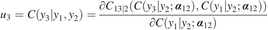
v. Continue until we obtain yNyN by setting uN = C(yN| yN − 1, yN − 2, …yN − K; α)uN=CyNyN−1yN−2…yN−Kα.


Now, we have simulated the desired Kth-order Markov process in the frequency domain. Again, similar to the simulation of the first-order Markov model, the sequence simulated in the frequency domain needs to be transformed into the real-domain through either parametric marginal distribution or nonparametric marginal distribution (e.g., empirical distribution using plotting-position formulas and kernel density) with proper interpolation.
9.5.5 Forecast and Quantile Estimation of Kth-order Copula-Based Markov Models
For the Kth-order copula-based Markov process, the first-order median forecast formula (i.e., Equation (9.19)) can be rewritten as follows:
 (9.27)
Replacing the unknown true marginal distribution (F∗F∗) by its nonparametric marginal distribution (FnFn), and true copula parameter vector αα by the estimated parameter α̂ , Equation (9.27) can be rewritten as follows:
 (9.27a)
Similar to Equation (9.19a), Equation (9.27a) of the conditional probability (also called the conditional copula) of Zt ∣ Zt − 1 = zt − 1, …, Zt − K = zt − KZt∣Zt−1=zt−1,…,Zt−K=zt−K is equal to 0.5 (also called the 50% conditional quantile). The median forecast can be computed using the following:
 (9.28)
Furthermore, for any given conditional quantile q, its associated time series value may be computed using the following:
 (9.29)
Example 9.4 Rework TS2 series in Example 9.2 using (i) meta-Gaussian and (ii) Frank copulas. Also, compare the results with those from AR(2) model in Example 9.2.
Solution: According to Example 9.2, the time series TS2 is fitted with the classic AR(2) model. We will proceed with the following procedure:
i. Identify the Markov order for the time series:
Lag-1 dependence: To assess the lag-1 dependence (i.e., TS2t and TS2t − 1)TS2tandTS2t−1), we will simply compute the rank-based Kendall correlation coefficient and assess its significance (using the critical value of α = 0.05)α=0.05).
Using Equation (3.68) (or simply using the MATLAB function corr), we compute the following:
τnLag1=0.5765,Pvalue≤10−4Results show that the lag-1 dependence is significant.
Lag-2 dependence: To assess the lag-2 dependence (i.e., TS2t and TS2t − 2TS2tandTS2t−2), we need to evaluate the dependence of Ft ∣ t − 1(zt| zt − 1)Ft∣t−1ztzt−1 and Ft − 2 ∣ t − 1(zt − 2| zt − 1)Ft−2∣t−1zt−2zt−1. Thus, we first need to estimate the conditional distribution (or simply conditional copula) with the understanding that {zt, zt − 1}ztzt−1 and {zt − 1, zt − 2zt−1,zt−2} have the same copula. Using meta-Gaussian copula, we can simply estimate the copula parameter through Kendall’s tau, previously computed as follows:
ρ=sinπ2τnlag1=0.7868We now build the bivariate Gaussian copula for the lag-1 sequence and compute the corresponding conditional copulas. The conditional copula results are listed in Table 9.9. The Kendall correlation coefficient is computed as follows:
Now, we conclude that lag-2 dependence is still significant. We will need to move on to the evaluation of lag-3 dependence.
τn[F(zt| zt − 1), F(zt − 2| zt − 1)] = − 0.2748, Pvalue≈0.006τnFztzt−1Fzt−2zt−1=−0.2748,Pvalue≈0.006
Lag-3 dependence: Similar to the lag-2 dependence assessment, we will need to evaluate the rank-based conditional dependence of the following: {F(zt| zt − 1, zt − 2), F(zt − 3| zt − 1, zt − 2)}Fztzt−1zt−2Fzt−3zt−1zt−2
In the preceding formulation, we can further write the two components using Equation (5.24) as follows:
Fztzt−1zt−2=∂Czt,zt−2∣zt−1Czt∣zt−1Czt−2∣zt−1∂Czt−2∣zt−1 (9.30a)
Fzt−3zt−1zt−2=∂Czt−3,zt−1∣zt−2Czt−3∣zt−2Czt−1∣zt−2∂Czt−1∣zt−2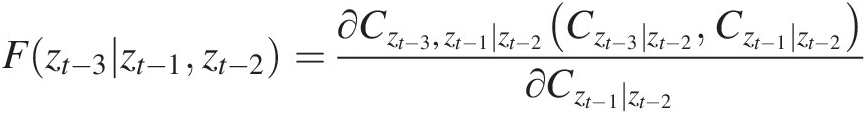 (9.30b)
To compute the conditional probability for Equations (9.30a) and (9.30b), we apply the meta-Gaussian copula first using the Gaussian copula fitted to the lag-2 dependence assessment. The conditional distribution for Czt ∣ zt − 1, Czt − 2 ∣ zt − 1, Czt − 1 ∣ zt − 2, Czt − 3 ∣ zt − 2Czt∣zt−1,Czt−2∣zt−1,Czt−1∣zt−2,Czt−3∣zt−2 is also listed in Table 9.10.
With these conditional probabilities computed, we estimate the copula parameters for Czt, zt − 2 ∣ zt − 1, Czt, zt − 2 ∣ zt − 1Czt,zt−2∣zt−1,Czt3,t1jt2 that are –0.45 and –0.42 respectively. Now, we can compute F(zt| zt − 1, zt − 2), F(zt − 3| zt − 1, zt − 2)Fztzt−1zt−2,Fzt−3zt−1zt−2, which are again listed in Table 9.10. Now Kendall’s correlation coefficient is computed as follows:
τn[F(zt| zt − 1, zt − 2), F(zt − 3| zt − 1, zt − 2)] = 0.1674, Pvalue≈0.099>0.05τnFztzt−1zt−2Fzt−3zt−1zt−2=0.1674,Pvalue≈0.099>0.05
It is then concluded that it is reasonable to apply the second-order copula-based Markov process for the dataset.
ii. Estimate the parameters for the second-order copula-based Markov model.
From the results obtained in step i, we know that a trivariate copula will be needed to model the second-order Markov process for time series TS2, for which the schematic for the trivariate D-vine copula is shown in Figure 9.12. As given in the problem statement, the parameters of the meta-Gaussian, the Student t, and the Frank-vine copula structures will be estimated with the use of sequential parameter estimation.
Meta Gaussian vine copula structure:
In this case, we apply the meta-Gaussian copulas (Equation (7.40)) for T1 and T2. We will use the parameters estimated nonparametrically for lag-dependence evaluation as initial parameters.
T1: using ρin = 0.7868ρin=0.7868 for {zt, zt − 1}ztzt−1 & {zt − 1, zt − 2}zt−1zt−2 and applying the semiparametric MLE, we have the parameter estimated for the lag-1 serial dependence of T1 as ρT1 = 0.8265ρT1=0.8265.
T2. Fix the parameter estimated for T1 to compute the conditional copula of Ct ∣ t − 1, Ct − 1 ∣ t − 2Ct∣t−1,Ct−1∣t−2 (listed in Table 9.11). Finally, using the computed conditional copula of bivariate variables, we estimate the parameter for T2 as ρT2 = − 0.3879ρT2=−0.3961.
Frank vine copula structure:
Using the same procedure as that for the meta-Gaussian copula, we again estimate the parameters for the Frank copula (Copula No. 5, Table 3.1) using the semiparametric MLE as follows:
αT1 = 7.9422; αT2 = − 2.4461αT1=7.9422;αT2=−2.4461.
Again, the conditional copula needed for the parameter estimation for T2 is listed in Table 9.11.
iii. Simulate the univariate time series.
Compared to the simulation for the first-order copula-based Markov process, we will need to simulate variate y3y3 through Equation (9.30b). Following the simulation discussed in Section 9.5.4, Figure 9.13 shows simulations from the copula-based model as well as the simple AR(2) model. To further compare the classic AR(2) model to the second-order copula-based Markov model, we perform the one-step ahead forecast using exactly the same rationale as in Example 9.3.
One-step ahead forecast from AR(2): TS2̂51≈476.40
 .
.
One-step ahead forecast from the Gaussian copula-based second-order Markov model:
F̂TS251=0.7512;TS2̂51Gaussian=476.472

One-step ahead forecast from the Frank copula-based second-order Markov model:
F̂TS251=0.7719;TS2̂51Gaussian=476.562

From the forecast results, it is seen that there is minimal difference between the classic AR(2) model and copula-based models. Given the time series data applied in Examples 9.2 and 9.4 as the synthetic time series generated from the AR(2) model, it is no surprise that overall the Gaussian copula-based model performs more similarly to the AR(2) model. Figure 9.14 plots the scatter plots for the lag-1 and lag-2 dependences. Figure 9.14 shows that the copula-based Markov model captures the serial dependence well.


Figure 9.12 Vine-copula structure for the second-order copula-based Markov process.

Figure 9.13 Simulations from AR(2) and copula-based second-order Markov models.
Table 9.10. Markov order identification results table.
| Time series | Lag-2 | Lag-3 | |||||||
|---|---|---|---|---|---|---|---|---|---|
| TS2 | CDF | (1) | (2) | (3) | (4) | (5) | (6) | (7) | (8) |
| τ≈ − 0.27τ≈−0.27 P≈0.0056P≈0.0056 | τ≈0.1674τ≈0.1674 P≈0.099P≈0.099 | ||||||||
| 476.35 | 0.72 | ||||||||
| 475.48 | 0.49 | ||||||||
| 476.02 | 0.64 | 0.72 | 0.84 | ||||||
| 476.75 | 0.81 | 0.84 | 0.32 | 0.84 | 0.32 | 0.72 | 0.84 | 0.81 | 0.91 |
| 476.89 | 0.84 | 0.68 | 0.29 | 0.68 | 0.29 | 0.84 | 0.32 | 0.60 | 0.47 |
| 477.27 | 0.90 | 0.79 | 0.57 | 0.79 | 0.57 | 0.68 | 0.29 | 0.83 | 0.34 |
| 477.51 | 0.93 | 0.76 | 0.50 | 0.76 | 0.50 | 0.79 | 0.57 | 0.79 | 0.71 |
| 476.50 | 0.76 | 0.24 | 0.59 | 0.24 | 0.59 | 0.76 | 0.50 | 0.25 | 0.63 |
| 475.87 | 0.60 | 0.31 | 0.93 | 0.31 | 0.93 | 0.24 | 0.59 | 0.57 | 0.47 |
| 475.74 | 0.56 | 0.47 | 0.80 | 0.47 | 0.80 | 0.31 | 0.93 | 0.63 | 0.91 |
| 475.29 | 0.45 | 0.34 | 0.58 | 0.34 | 0.58 | 0.47 | 0.80 | 0.36 | 0.81 |
| 476.75 | 0.81 | 0.95 | 0.66 | 0.95 | 0.66 | 0.34 | 0.58 | 0.98 | 0.51 |
| 476.60 | 0.78 | 0.55 | 0.09 | 0.55 | 0.09 | 0.95 | 0.66 | 0.30 | 0.89 |
| 475.69 | 0.55 | 0.21 | 0.67 | 0.21 | 0.67 | 0.55 | 0.09 | 0.25 | 0.08 |
| 474.94 | 0.37 | 0.24 | 0.86 | 0.24 | 0.86 | 0.21 | 0.67 | 0.41 | 0.55 |
| 473.83 | 0.19 | 0.15 | 0.73 | 0.15 | 0.73 | 0.24 | 0.86 | 0.20 | 0.81 |
| 473.63 | 0.16 | 0.31 | 0.72 | 0.31 | 0.72 | 0.15 | 0.73 | 0.40 | 0.59 |
| 473.84 | 0.19 | 0.43 | 0.43 | 0.43 | 0.43 | 0.31 | 0.72 | 0.39 | 0.67 |
| 475.58 | 0.52 | 0.89 | 0.31 | 0.89 | 0.31 | 0.43 | 0.43 | 0.87 | 0.39 |
| 476.17 | 0.68 | 0.75 | 0.07 | 0.75 | 0.07 | 0.89 | 0.31 | 0.50 | 0.51 |
| 475.11 | 0.40 | 0.16 | 0.31 | 0.16 | 0.31 | 0.75 | 0.07 | 0.09 | 0.09 |
| 476.29 | 0.71 | 0.88 | 0.85 | 0.88 | 0.85 | 0.16 | 0.31 | 0.97 | 0.16 |
| 478.09 | 0.97 | 0.99 | 0.14 | 0.99 | 0.14 | 0.88 | 0.85 | 0.98 | 0.96 |
| 478.04 | 0.97 | 0.72 | 0.07 | 0.72 | 0.07 | 0.99 | 0.14 | 0.46 | 0.45 |
| 476.20 | 0.68 | 0.06 | 0.76 | 0.06 | 0.76 | 0.72 | 0.07 | 0.08 | 0.08 |
| 475.13 | 0.41 | 0.16 | 0.99 | 0.16 | 0.99 | 0.06 | 0.76 | 0.53 | 0.52 |
| 475.01 | 0.38 | 0.43 | 0.86 | 0.43 | 0.86 | 0.16 | 0.99 | 0.63 | 0.98 |
| 475.44 | 0.48 | 0.62 | 0.50 | 0.62 | 0.50 | 0.43 | 0.86 | 0.63 | 0.86 |
| 475.49 | 0.49 | 0.51 | 0.34 | 0.51 | 0.34 | 0.62 | 0.50 | 0.43 | 0.56 |
| 475.91 | 0.61 | 0.68 | 0.48 | 0.68 | 0.48 | 0.51 | 0.34 | 0.69 | 0.33 |
| 476.52 | 0.76 | 0.79 | 0.35 | 0.79 | 0.35 | 0.68 | 0.48 | 0.76 | 0.56 |
| 475.51 | 0.50 | 0.18 | 0.32 | 0.18 | 0.32 | 0.79 | 0.35 | 0.10 | 0.48 |
| 474.24 | 0.25 | 0.13 | 0.88 | 0.13 | 0.88 | 0.18 | 0.32 | 0.25 | 0.18 |
| 473.57 | 0.15 | 0.21 | 0.81 | 0.21 | 0.81 | 0.13 | 0.88 | 0.32 | 0.78 |
| 473.33 | 0.12 | 0.28 | 0.58 | 0.28 | 0.58 | 0.21 | 0.81 | 0.30 | 0.72 |
| 473.42 | 0.13 | 0.37 | 0.42 | 0.37 | 0.42 | 0.28 | 0.58 | 0.32 | 0.49 |
| 473.87 | 0.19 | 0.50 | 0.32 | 0.50 | 0.32 | 0.37 | 0.42 | 0.41 | 0.36 |
| 471.65 | 0.03 | 0.03 | 0.24 | 0.03 | 0.24 | 0.50 | 0.32 | 0.01 | 0.31 |
| 470.84 | 0.01 | 0.11 | 0.84 | 0.11 | 0.84 | 0.03 | 0.24 | 0.19 | 0.05 |
| 472.87 | 0.08 | 0.71 | 0.42 | 0.71 | 0.42 | 0.11 | 0.84 | 0.70 | 0.70 |
| 473.17 | 0.10 | 0.41 | 0.03 | 0.41 | 0.03 | 0.71 | 0.42 | 0.12 | 0.51 |
| 474.16 | 0.23 | 0.66 | 0.24 | 0.66 | 0.24 | 0.41 | 0.03 | 0.55 | 0.02 |
| 475.32 | 0.45 | 0.77 | 0.13 | 0.77 | 0.13 | 0.66 | 0.24 | 0.60 | 0.28 |
| 475.63 | 0.53 | 0.61 | 0.15 | 0.61 | 0.15 | 0.77 | 0.13 | 0.42 | 0.19 |
| 475.90 | 0.60 | 0.63 | 0.38 | 0.63 | 0.38 | 0.61 | 0.15 | 0.58 | 0.16 |
| 474.64 | 0.31 | 0.13 | 0.42 | 0.13 | 0.42 | 0.63 | 0.38 | 0.08 | 0.43 |
| 474.19 | 0.24 | 0.30 | 0.85 | 0.30 | 0.85 | 0.13 | 0.42 | 0.48 | 0.23 |
| 476.01 | 0.63 | 0.93 | 0.54 | 0.93 | 0.54 | 0.30 | 0.85 | 0.95 | 0.82 |
| 476.85 | 0.83 | 0.87 | 0.06 | 0.87 | 0.06 | 0.93 | 0.54 | 0.68 | 0.79 |
| 476.79 | 0.82 | 0.60 | 0.25 | 0.60 | 0.25 | 0.87 | 0.06 | 0.48 | 0.11 |
Note: Lag-2: (1) F(zt| zt − 1)Fztzt−1; (2) F(zt − 1| zt − 2)Fzt−1zt−2
Lag-3: (3) F(zt| zt − 1)Fztzt−1; (4) F(zt − 2| zt − 1)Fzt−2zt−1; (5) F(zt − 1| zt − 2)Fzt−1zt−2; (6) F(zt − 3| zt − 2)Fzt−3zt−2
(7) F(zt| zt − 1, zt − 2)Fztzt−1zt−2; (8) F(zt − 3| zt − 1, zt − 2)Fzt−3zt−1zt−2
Table 9.11. Parameter estimation results.
| Time series | Meta-Gaussian | Frank | ||||
|---|---|---|---|---|---|---|
| Lag-2 | Lag-1 | TS2 | Ct ∣ t − 1Ct∣t−1 | Ct − 2 ∣ t − 1Ct−2∣t−1 | Ct ∣ t − 1Ct∣t−1 | Ct − 2 ∣ t − 1Ct−2∣t−1 |
| (t−2) | (t−1) | t | ρlag1 = 0.8265ρlag1=0.8265 | θlag1 = 7.9422θlag1=7.9422 | ||
| NaN | NaN | 0.72 | ||||
| NaN | 0.72 | 0.49 | ||||
| 0.72 | 0.49 | 0.64 | 0.74 | 0.86 | 0.77 | 0.87 |
| 0.49 | 0.64 | 0.81 | 0.86 | 0.29 | 0.84 | 0.24 |
| 0.64 | 0.81 | 0.84 | 0.68 | 0.25 | 0.63 | 0.21 |
| 0.81 | 0.84 | 0.90 | 0.79 | 0.55 | 0.74 | 0.51 |
| 0.84 | 0.90 | 0.93 | 0.76 | 0.46 | 0.74 | 0.47 |
| 0.90 | 0.93 | 0.76 | 0.19 | 0.55 | 0.24 | 0.59 |
| 0.93 | 0.76 | 0.60 | 0.28 | 0.94 | 0.22 | 0.89 |
| 0.76 | 0.60 | 0.56 | 0.46 | 0.81 | 0.43 | 0.81 |
| 0.60 | 0.56 | 0.45 | 0.32 | 0.58 | 0.28 | 0.58 |
| 0.56 | 0.45 | 0.81 | 0.96 | 0.68 | 0.96 | 0.72 |
| 0.45 | 0.81 | 0.78 | 0.53 | 0.06 | 0.49 | 0.05 |
| 0.81 | 0.78 | 0.55 | 0.18 | 0.67 | 0.14 | 0.62 |
| 0.78 | 0.55 | 0.37 | 0.22 | 0.88 | 0.19 | 0.88 |
| 0.55 | 0.37 | 0.19 | 0.14 | 0.76 | 0.15 | 0.81 |
| 0.37 | 0.19 | 0.16 | 0.32 | 0.76 | 0.37 | 0.80 |
| 0.19 | 0.16 | 0.19 | 0.45 | 0.45 | 0.49 | 0.49 |
| 0.16 | 0.19 | 0.52 | 0.92 | 0.32 | 0.93 | 0.36 |
| 0.19 | 0.52 | 0.68 | 0.77 | 0.05 | 0.79 | 0.05 |
| 0.52 | 0.68 | 0.40 | 0.14 | 0.28 | 0.10 | 0.22 |
| 0.68 | 0.40 | 0.71 | 0.91 | 0.88 | 0.93 | 0.90 |
| 0.40 | 0.71 | 0.97 | 0.99 | 0.11 | 0.97 | 0.08 |
| 0.71 | 0.97 | 0.97 | 0.69 | 0.04 | 0.81 | 0.12 |
| 0.97 | 0.97 | 0.68 | 0.03 | 0.74 | 0.10 | 0.83 |
| 0.97 | 0.68 | 0.41 | 0.13 | 0.99 | 0.10 | 0.98 |
| 0.68 | 0.41 | 0.38 | 0.43 | 0.88 | 0.44 | 0.91 |
| 0.41 | 0.38 | 0.48 | 0.64 | 0.51 | 0.69 | 0.54 |
| 0.38 | 0.48 | 0.49 | 0.52 | 0.32 | 0.52 | 0.30 |
| 0.48 | 0.49 | 0.61 | 0.69 | 0.48 | 0.72 | 0.47 |
| 0.49 | 0.61 | 0.76 | 0.81 | 0.33 | 0.80 | 0.29 |
| 0.61 | 0.76 | 0.50 | 0.15 | 0.29 | 0.11 | 0.23 |
| 0.76 | 0.50 | 0.25 | 0.11 | 0.90 | 0.10 | 0.90 |
| 0.50 | 0.25 | 0.15 | 0.20 | 0.84 | 0.24 | 0.88 |
| 0.25 | 0.15 | 0.12 | 0.29 | 0.62 | 0.33 | 0.65 |
| 0.15 | 0.12 | 0.13 | 0.39 | 0.45 | 0.41 | 0.47 |
| 0.12 | 0.13 | 0.19 | 0.53 | 0.33 | 0.55 | 0.36 |
| 0.13 | 0.19 | 0.03 | 0.02 | 0.24 | 0.05 | 0.29 |
| 0.19 | 0.03 | 0.01 | 0.11 | 0.89 | 0.08 | 0.74 |
| 0.03 | 0.01 | 0.08 | 0.78 | 0.47 | 0.44 | 0.19 |
| 0.01 | 0.08 | 0.10 | 0.44 | 0.03 | 0.41 | 0.05 |
| 0.08 | 0.10 | 0.23 | 0.71 | 0.25 | 0.70 | 0.27 |
| 0.10 | 0.23 | 0.45 | 0.80 | 0.12 | 0.85 | 0.17 |
| 0.23 | 0.45 | 0.53 | 0.63 | 0.13 | 0.66 | 0.13 |
| 0.45 | 0.53 | 0.60 | 0.64 | 0.37 | 0.65 | 0.34 |
| 0.53 | 0.60 | 0.31 | 0.10 | 0.40 | 0.08 | 0.36 |
| 0.60 | 0.31 | 0.24 | 0.29 | 0.88 | 0.32 | 0.91 |
| 0.31 | 0.24 | 0.63 | 0.95 | 0.57 | 0.96 | 0.62 |
| 0.24 | 0.63 | 0.83 | 0.89 | 0.04 | 0.87 | 0.04 |
| 0.63 | 0.83 | 0.82 | 0.59 | 0.21 | 0.55 | 0.18 |

Figure 9.14 Lag-1 and lag-2 dependence comparison of simulated time series to the orginal time series TS2.
9.6 Summary
This chapter further reveals the advantages of the copula theory not only in traditional frequency analysis but also in time series analysis:
i. It allows the investigation of spatial and temporal dependences separately from their marginals and their effect.
ii. It is more robust for to modeling any type of temporal (serial dependence) and avoids the Gaussian process assumption of the time series modeling approach.
iii. It provides a better approach to identify the necessary order for the Markov process.
iv. Vine copula may be easily applied to model a higher-order Markov process.
v. These advantages are very important for the hydrological analysis under the impact of climate change and land use/land cover (LULC) when the univariate hydrological variables may no longer be considered as independent random variables.