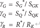
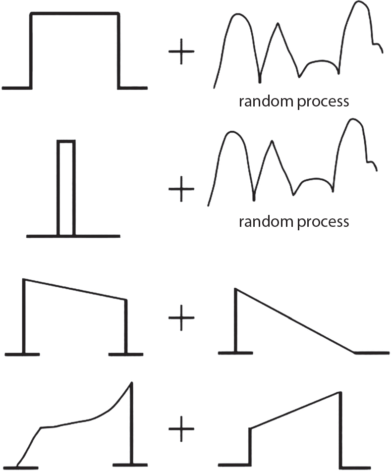
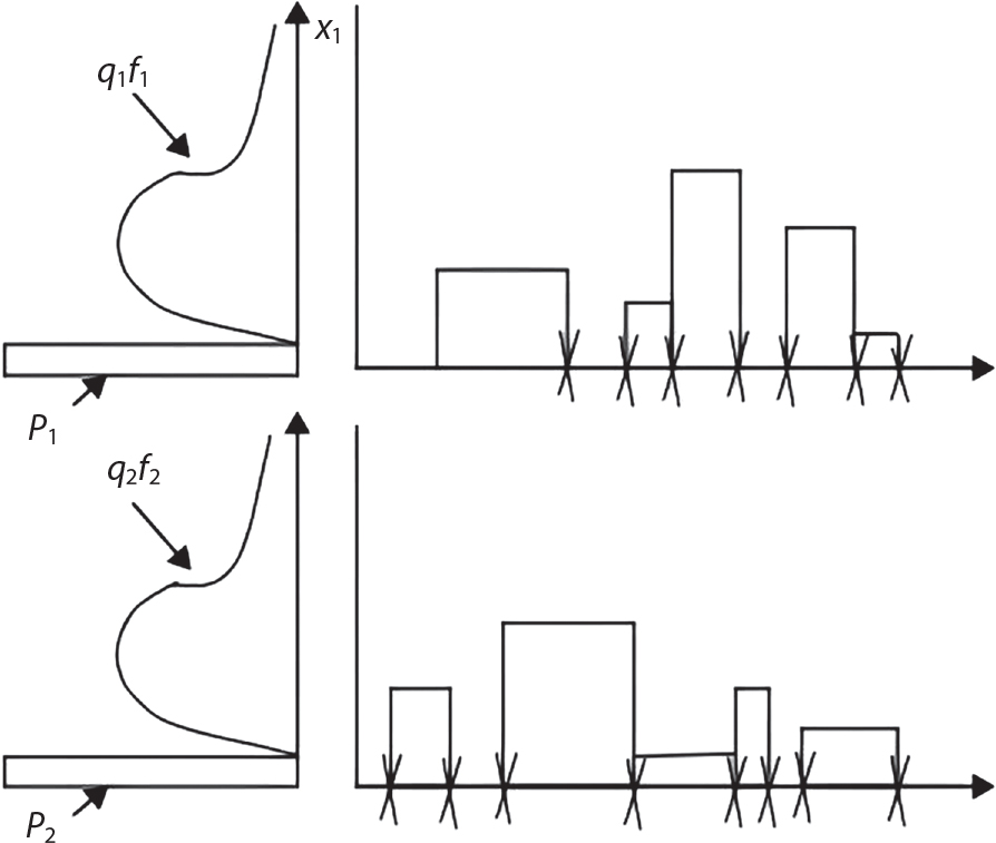
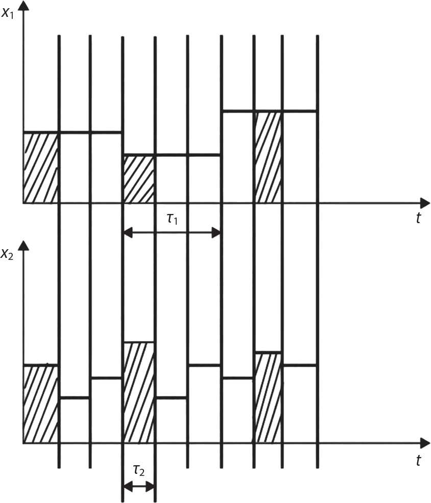
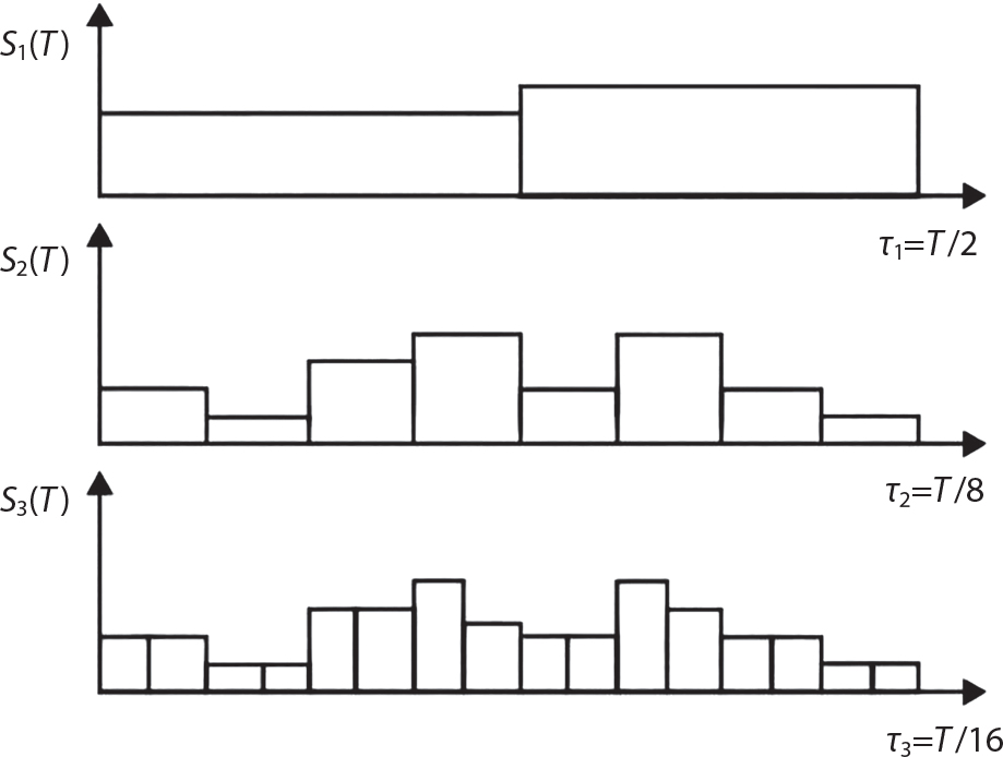
Random load combination plays an important role in engineering structural design theory, and especially in reliability theory. Loads are combined to find an equivalent load to replace two or more random processes acting on the structure. The load combination rule provided in the code should be simple enough to facilitate engineering application. The combination rule is mainly based on the time integral method. The rule of simplification will be discussed in the next chapter. If X1(t) and X2(t) represent stationary, mutually independent and continuous load random processes, the probability distribution of the linear combination X = X1 + X2 in the time interval [0, tL] can be calculated by considering the transcending rate of X(t) with respect to the horizontal line x = a in Equation (7.1). The major problem involves calculating the transcending rate of horizontal a, X, or the crossing rate at which (X1, X2) leaves the area enclosed by the plane x1 + x2 = a. where v is average cross rate of event occurrence. If both X1(t) and X2(t) are normal random processes, while X = X1 + X2 is also normal and stationary, then the mean and variance can be calculated. For the crossing rate v of stationary normal random processes, these can be directly obtained from the results of a single random process in Equation (7.2). Unfortunately, not all load random processes can be properly described. For example, sufficient accuracy cannot be ensured for transient normal random processes or the application of Equation (7.3) to non-normal process calculation. Generally, the crossing rate of random processes can be calculated by Equation (7.4). The joint probability density function (PDF) where It is usually difficult to obtain an analytical solution. Once the integral domain of where vi(u) represents the crossing rate of random process Xi(t) at the transcending rate of horizontal u. Equation (7.7) offers a solution to the combination of random processes, especially when the random processes X1(t) and X2(t) obey a discrete distribution. Equation (7.7) also may apply to the combinations of random processes that satisfy: Figure 7.1 shows typical random processes that are consistent with this situation. If both X1(t) and X2(t) are stationary normal random processes, with a mean of The crossing rate of each independent random process can be obtained from: Figure 7.1 The combination of random process. After the above results are substituted into Equation (7.7), the upper limit of crossing rate of X = X1 + X2 is turned into: where Let’s consider a combination of two non-negative rectangular update processes. Figure 7.2 shows a typical trajectory (or implementation) chart. The crossing rate of each random process can be calculated: where the mean arrival rate of the random pulses is viqi = vmi, the distribution at any time point is Figure 7.2 Typical sample function of mixed rectangular update stochastic process with given probability density function. Fortunately, this result is very simple to explain, and can be solved using the most basic theory. For a random process, if the X(t) value is non-negative whenever it is updated, then the probability value is q. Similarly, when the X(t) value is 0, the probability value is p, regardless of the X(t) value within the current time increment. Therefore, the random process has no aftereffect. Table 7.1 shows various possible states of transcending level a after two random processes are combined. The effect of each state change (e.g., from X1 + X2 < a to X1 + X2 > a) on the crossing rate Table 7.1 Different state combinations that cause crossing. Let Ω = •State Change Δt•. So, the term (a) in Table 7.1 becomes: or The above formula is consistent with the second term in Equation (7.11) because v2q2 = vm2. The term (b) in Table 7.1 becomes: or The above formula is consistent with the fourth term in Equation (7.11) (v2q2 = vm2). The term (c) in Table 7.1 is turned into: or The above formula is equal to the sixth term in Equation (7.11). Other terms in Equation (7.11) change with the change of states (d)∼(f) in Table 7.1. If each pulse returns to zero before the start of the next pulse, then the term p2 + q2F2(a) in Equation (7.13) is equal to 1 by definition, and the same is true for the term p2 in Equation (7.14). If the crossing rate is obtained by calculation, then the cumulative distribution function (CDF) FX( ) of load X = X1 + X2 can be obtained by calculation using Equation (7.1). Some academic researchers have studied the calculation error between Equation (7.1) and Equation (7.2). By comparing with certain known exact solutions [7-3][7-4][7-5][7-6], we find that the calculation error for a high-level obstacle a is 20%, while the calculation error for a low-level obstacle is 60%. (1) Directional simulation in load effect space The load in pulse mode can be simplified by Equation (7.11). For example, let where G12( ) = 1 − F12( ), F12( ) is the CDF between two pulses. So, Equation (7.11) can be simplified to: where vmiμi is replaced with qi. vmi represents the average pulse arrival rate of random process Xi(t). μi represents the duration of pulse Xi(t). If the duration is short enough, i.e., μi → 0, and the relative probability of its occurrence is very low, then pi → 1. The crossing rate of combined random processes can be approximated to: This equation was first proposed by Wen [7-7]. The first and second terms in Equation (7.17) represent the crossing rate when each random process acts alone, while the third term represents the crossing rate when two random processes act simultaneously (i.e., pulse overlapping). The third term can be ignored if the pulse duration is very short. The existing research shows that, compared with the simulation results, Equation (7.17) can be used to accurately estimate the crossing rate (2) Borges processes The combination of Borges processes is of particular significance for code validation, because it helps to accurately estimate the maximum combination effect of load probability distribution [7-11]. When every random process Xi(t) in the random process combination X = X1 + X2 + X3 +⋯ is a Borges process, then the pulse duration is τ1 < τ2 < τ3 < …, and τi / τi−1 is an integer. See Figure 7.3. Therefore, the occurrence rate is equal to the number ni of pulses in the random process Xi during the time interval [0, tL] divided by the duration, i.e., vi = ni / tL. According to the above crossing rate formula, the CDF of the maximum value of X can be obtained by Equation (7.1). However, another method will also be briefly introduced below. The CDF Fmax X( ) of maximum X can be calculated by convolution computation in the equation below [7-12]: Figure 7.3 Borges process combination. The above formula is a bivariate random process, τ2 = τ1 / m, where m is an integer, and there are n pulses about τ1 within [0, tL]. For a combination of two or more loads, this integral term is more complex, but a calculation can be performed using the first-order second-moment method. For a linear combination of three loads, the maximum value within [0, tL] can be written as: where Z2(t) is expressed as: where The CDF where where If the supplementary terms to all the random processes in The mean (3) Deterministic load combination—Turkstra’s combination rule Many simplified methods are used for load combination calculations, but they are still very complicated for conventional structural design and code formulation. The most basic load combination method is to add up the loads directly without considering the uncertainty of these loads. Then, a series of coefficients are proposed to amplify or reduce the loads to an appropriate extent. The key problem is how to ensure the rationality of these coefficients. Load combination rules can be extracted from a combination of Borges processes [7-13] or from Equation (7.7). If the approximation where the maximum value is taken over the entire time interval concerned, such as the service life [0, tL] of the structure. For combination Z = W + V, where W and V are independent of each other, the CDF GZ( ) can be obtained by means of the convolution integral: Therefore, the two integrals in Equation (7.23) represent max For a high failure level a, the last item can be ignored, so This is the famous Turkstra combination rule. It can be expressed as: (1) The sum of the maximum value of Load 1 within the service life and the value of Load 2 taken when Load 1 reaches its maximum value; (2) The sum of the maximum value of Load 2 within the service life and the value of Load 1 taken when Load 2 reaches its maximum value. This combination rule can be extended to a combination of multiple loads or multiple load effects. For a combination of n loads: This combination is analogous to the load combination rules specified in the current codes, and obviously, is also related to the probability theory requirements in load combination. However, the load level is not specified in Turkstra’s combination rule, but needs to be selected one by one. Chapter 8 will describe that if the random process Xi is stationary, then the value of [max Xi] is usually equal to 95% of the load, and Although Turkstra’s combination rule is very simple to apply to standardized engineering applications, it is not very suitable for probability calculations that have high requirements for accuracy. Load or load effect is a decisive factor in structural design, and its load combination is one of the core issues, running right the way through reliability design standards. For a structure that bears n loads, if the time-dependent change of structural resistance is ignored, then its limit state equation can be expressed as where R represents structural resistance, Si(t) represents the random process of the ith load effect, and S(t) represents the random process of the combined effect of n loads. Obviously, the key problem in structural reliability analysis is load combination. From a mathematical perspective, the problem of load combination involves the superposition of multiple random processes. In engineering practice, the random processes are generally replaced with the maximum load in the reference period (a variable random), for reliability analysis. Therefore, the key to load combination is to determine the maximum value SM of load combination, as follows The theory and rules of random load combination include [7-14] (i) peak superposition; (ii) crossing analysis; (iii) combinatorial theory Poisson process as a simplified model; (iv) maximum value formed by the local extreme values of certain time intervals from the perspective of engineering practice; and (v) square root of the sum of the squares (SRSS). This method assumes that all load processes reach a maximum simultaneously, with these maximum values added up to obtain the designed value. This is the most conservative combination model. Actually, it should be considered as a deterministic analysis method. Currently, this method is often used for offshore structure design. The up-crossing theory has been used by many academic researchers to study nonlinear or dynamic load combination problems. Let X(t) be a stationary random process, implemented as x(t) in t1,t2. Given a constant threshold value X(t) = r, as shown in the figure, the up-crossing level X(t) is called positive crossing, which is marked in the figure. The derivative process The step function H(x) needs to be used to derive the up-crossing rate theory, and it is defined by Heaviside, i.e., For random process X(t) and fixed threshold x(t) = r, we define so then For the number of such unit pulses in the time interval [t1,t2], the total number of times the threshold level x(t) = r is crossed can be obtained as follows The average number of all pulses in time interval [t1,t2] is as follows: Consider the positive crossing rate per unit time, and let N(r, t). Then so The average crossing rate (also called up-crossing rate) per unit time is as follows: Taking two random processes as an example, let X1(t) and X2(t) be independent continuous processes, then the probability distribution of X = X1 + X2 in [0, t] can be obtained according to the assumption that its up-crossing obeys the Poisson distribution where υ(x, t) represents the up-crossing rate corresponding to the threshold at t. If X1,X2 are stationary random processes, then υ(x, t) = υ(x), and υ(x) can be expressed by an integral, i.e., This method is based on a combined model of Poisson processes, first proposed by Hasofer [7-15], who assumed that there should be a linear relationship between load and load effect, as follows: (1) Hasofer combination method. In this method, loads are divided into persistent variable loads (Class-a) and temporary variable loads (Class-b). If the distribution style and probability density of these two types of loads, as well as the average occurrence rate of load effects, are known, then the maximum distribution of Class-b load effects in the duration of Class-a loads can be obtained by probability theory. Then, the extreme value distribution of combined effects during the design reference period can be obtained. This method, which involves the computation of multiple continuous integrals, is not a mature approach in practice. (2) Wen combination method [7-16][7-17] [7-18] [7-19]. It is basically the same idea as the Hasofer combination method. There is a great difference between Class-a and –b effects in terms of frequency and duration. If the average occurrence rate of the ith effect is υi, and the average duration is where Gi(X) = 1 − Fi(X), Gij(X) = 1 − Fij(X), Gijk(X) = 1 − Fijk(X), where Fi(X) is the distribution function of load I; Fij(X) and Fijk(X) are, respectively, the probability distribution functions of loads I and j and the combination of I, j and k. υij and υijk represent the average meeting rate of I and j, as well as I, j and k, respectively. After further simplification, the maximum post-combination distribution can be obtained by a mathematical method. Although such methods feature a reasonable combination type, they require complete observed and statistical data, such as the average occurrence rate of loads. These tend to be difficult to obtain in practice. Moreover, the calculation process is complex, making it difficult to apply them to ocean engineering designs. In a linear system, the maximum/RMS value is approximately identical at time T for all responses, while the period and frequency are independent of each other, so where peak factor It is simple to adopt this combination, i.e., This kind of method is not designed to calculate the probability distribution of the maximum value of the combined effect from the perspective of mathematical logic. Rather, it is used to work out the actual maximum value of the combined effect generated on the envelope structure based different combinations of the local extreme values of a single effect taken in a specific time intervals. Common combination rules are as follows. (1) Turkstra’s rule for random load combination [7-20] [7-21] This is the combination model recommended in American National Standard A58. At present, this method has been adopted in the Unified Standard for Reliability Design of Hydraulic Engineering Structures [7-22] (GB50199-94) and the Unified Standard of Reliability of Structure Design for Harbor Engineering [7-23] (GB50158-92). According to the first load combination rule to be proposed by Turkstra, the extreme value of a load effect in [0, T] can be combined with the instantaneous value of the remaining load effects in turn, after which the combination with the largest load effect is selected as a control form. The combined maximum is then as follows: where t0 represents the moment at which Si(t) reaches its maximum, as shown in Figure 7.4. Figure 7.4 shows three different loading processes. According to Turkstra’s principle, the combined maximum to be evaluated is determined by the most unfavorable of the three combinations. The distribution function of the combined maximum is as follows: where Figure 7.4 TR combination diagram of three load combinations. (2) Ferry Borges-Castanheta rule for random load combinations The combination rule is an iso-temporal load combination model, proposed in 1972 by Ferry Borges and Castanheta[7-24], with reference to Turkstra’s rule. According to this combination rule, for every variable load xi, it can be divided into ri equal sections τi, which are then used as basis intervals throughout the service life of the structure, T. In each time interval, xi(t) does not change with time, xi(t) is statistically independent in sequential time intervals, and the probability of occurrence of xi(t) in each time interval is Pi. ri represents the number of repetitions of loads during the service life. For selection of τi, the maximum reached in sequential time intervals should be used to build an independent hypothesis. As can be seen from the above, the distribution of the maximum can be described using a stationary binomial process. So When considering a combination of several variable loads (random processes), we can assume that the random processes are independent of one another, and that the number of time intervals, ri, divided by time T, is an integer. Also, let When n=3, the Figure 7.5 shows three rectangular oscillo-grams simplified as equal time intervals. Figure 7.5 Process combination of three rectangular wave. Starting from the load xn that is repeated for the largest number of times, we work out the maximum xn(t, τn−1) of xn(t) in time interval τn−1, and obtain According to Equation (7.48), max(x1 + x2 + ⋯ + xn) can be approximated as max(x1 + x2 + ⋯ + xn−2 + Zn−1) so as to reduce the problem from a combination of n loads to a combination of (n-1) loads, where the distribution of Zn−1 is the convolution of the distribution function Equation (7.49) is the superposition process of this rule. Because Zi = xi+1(τi) + xi obtained by superposition each time is a constant maximum in this time interval, the results obtained are obviously more conservative, especially when n is larger. Besides, the sequential convolution operations in the previous formula are also very tedious. Figure 7.5 shows the superposition process of the F-B rule. There are three load effects, x1(t),x2(t),x3(t), where r1 < r2 < r3, and the combined maximum is shown in Equation (7.50): (3) JCSS combination rule for random load combination (pyramid method) This load effect combination model is recommended in Volume I [7-25][7-27] of the International System of Unified Standard for Structures issued by the International Joint Committee on Structural Safety (JCSS), composed of six international organizations. It is also a combined probability model of load effects adopted in China’s Unified Standard for Building Structures [7-26] [7-28]. This model can be used to combine load effects in accordance with engineering experience. This is compatible with the use of first-order second-moment method considering the probability distribution types of basic variables to analyze structural reliability. The main contents are: Where CQ is a coefficient of Q(t). where Si(t0) is a random variable at any time point of the ith load effect Si(t). (4) Comparison of common random load combination rules Three examples of live load combinations: persistent live load Li, temporary live load Lr and wind load W, are taken to compare the above random load combination rules. The specific data is shown in Table 7.2. The load meeting method, F-B combination, TR combination and JCSS combination of these three random loads at different load-effect ratios are calculated according to the above-mentioned random load combination theory. For the convenience of comparison, the combination results are achieved by the dimensionless ratio As can be seen from Figure 7.6, the calculation results of various combination rules vary greatly with the load-effect ratio SL/SW; when the load-effect ratio is 1, the minimum value is reached. The F-B combination rule boasts the largest calculation results, indicating that this combination method is more conservative. As can also be seen, the JCSS combination rule and TR combination rule are less conservative when the load-effect ratio is low, but become increasingly conservative as the load-effect ratio rises. Therefore, various combination rules differ from one another in terms of risk at different load-effect ratios. Table 7.2 Parameters of various random loads. Figure 7.6 Comparison of several combination rules. In engineering structure design, partial coefficients are adopted in the expression of limit state design in order that the designed structure has the specified reliability. These coefficients are called partial coefficients of engineering structure design. According to the probability limit state design theory, there are load partial coefficients (including dead load and variable load) and resistance partial coefficients in the expression of engineering limit state design. The material properties, coefficient of variation of geometric parameters and uncertainty of resistance calculation model in the design expression are all included in resistance partial coefficients. The uncertainty of load calculation models is also included in load partial coefficients. The purpose of determining design partial coefficients is to implement the target reliability index of the engineering structure to each partial coefficient in the limit state design expression, so that complex numerical operations of probability limit states can be converted into a simple algebraic operation. When determining the partial coefficients in the limit state design expression, we must consider the type of load combination, the type of components, extreme working conditions, marine environmental loads, and the relevant statistical characteristics of structural resistance. Now, let’s show how partial coefficients are determined for the common load combination form, i.e., (dead load + live load). According to the limit state expression: At checking point X⋆, the limit state equation is written as: where According to the analysis of the structural reliability index, the determination of design partial coefficients is the inverse operation of the structural reliability index calculation. Therefore, we must use the relevant standard value and partial coefficients to replace the basic variables in the probability limit state equation at design checking point X⋆, as follows where SGK, SQK and RK are the standard value of dead load, the standard value of live load and the standard value of the resistance of structural components, respectively; γG, γQ and γR are partial coefficients of dead load, live load and resistance of structural components, respectively. Therefore, the following conditions must be met: From the foregoing explanation, the partial coefficients γG, γQ and γR depend on the design checking point coordinates of load and resistance. According to the analysis of the structural reliability index, the checking coordinates are related to the reliability index, indicating that design partial coefficients are also related to the reliability index. In addition, the checking point coordinates and corresponding reliability index are both related to the ratio of the standard value of live load to that of dead load (ρ), suggesting that design partial coefficients are also related to ρ. However, in engineering practice, the ρ value is constantly changing. In other words, both design partial coefficients and the corresponding reliability index change with the ρ value in practical engineering. Obviously, this does not meet practical requirements. The optimum partial coefficient means that there is a minimum difference between the reliability index of the structure designed with this coefficient at different load-effect ratios ρ and the target reliability index. In other words, the value of the partial coefficient should be determined according to the principle that the difference between the standard value of structural resistance worked out by the expression of partial coefficients and the standard value of structural resistance are directly worked out by the target reliability index. To determine the partial coefficients of engineering structure design, we primarily consider two cases, i.e., the simple condition and the additional combination (a combination of three loads), and follow the principles below: Load partial coefficients γG and γQ are determined by considering a simple combination. Dead load and live load combinations are thoroughly calculated and analyzed in order to determine γG and γQ. In order that γG and γQ should be universally applicable to structural components made of various materials, representative structural components and load-effect ratios are selected as the basis for calculation and analysis. For example, the target reliability index is 2.6∼2.9, and the following four different methods are used to calculate γG and γQ. (1) Least squares method for standard value of resistance According to the given target reliability index, mean value and standard value of random loads, and the coefficient of variation of structural resistance, the mean μR of structural resistance can be worked out by the checking point method based on the limit state equation. Then, the standard value RK * of resistance can be worked out according to the statistical parameters. For a certain component, if the standard value RK* of resistance obtained by target reliability is equal to the standard value of resistance obtained by the limit state equation, i.e., RK* = RK, then the reliability index of the component designed by this limit state equation must be equal to the target reliability index. Therefore, the above principles for determining partial coefficients can be converted into conditions for minimizing Hi below: where The possible value ranges of partial coefficients for dead loads are γG =1.1, 1.2, 1.3, 1.4 and 1.5; the possible value ranges of partial coefficients for variable loads are γQ =1.1, 1.2, 1.3, 1.4, 1.5, 1.6. Therefore, there are 30 value ranges for γG and γQ. Given each value range of γG and γQ, for every structural component, the least squares method can be used to calculate the optimum resistance partial coefficient The size of the I value reflects the difference between the target reliability index and the implicit reliability index of the structural component designed according to the design expression containing this set of γG and γQ, and various optimized This method can be used to determine partial coefficients according to the principle of least squares. Essentially, this method is to fit the standard value (2) Least squares method for reliability index By this method, partial coefficients are determined according to the principle that the error between the structural reliability index in the limit state design expression and the target reliability index is minimized. where (3) Specification method 1 All the load partial coefficients obtained by Equations (7.57) and (7.58) are results of optimization within a certain range. The load partial coefficients obtained by calculation may be different from the partial coefficients commonly used by designers. Thus, inconvenience is caused for both engineering design and engineering practice. To ensure the continuity between new and old codes, a new method called “Specification Method 1” has been proposed in Figure 7.7: Under extreme conditions, the dead load coefficient is kept unchanged when the dead load and live load are combined, i.e., γG = 1.3. The resistance partial coefficients of all structural components are calculated by the principle of least squares. Under the condition that load coefficient is known, the live load coefficient can be changed to calculate the partial coefficients of resistance. This is consistent with both engineering practice and designers’ design habits. (4) Specification method 2 Specification Method 2 is basically the same as Specification Method 1. To ensure the continuity between the new and old codes, four common resistance partial coefficients are known, i.e., axial compression is 0.85, axial tension is 0.95, bending is 0.95, and shearing is 0.95, to calculate load partial coefficients. Then, other resistance partial coefficients are calculated under the condition that load partial coefficients are known in Figure 7.8. Four common resistance partial coefficients are known in this method to calculate the partial coefficients of load and resistance. This is consistent with accepted engineering practice and design norms. Figure 7.7 Flow chart of specification method 1. Figure 7.8 Flow chart of specification method 2. (5) Method for determining resistance partial coefficients As mentioned earlier, during the process of selecting an optimal partial coefficient of load, given each set of γG and γQ, for every component i, under the condition that Hi is minimized, the least squares method can be used to determine an optimal partial coefficient resistance, where Sj = γG(SG)j +γQ(SQ)j, and the condition that ∂Hi/∂γi = 0 must be met. So Sj and In addition to dead load, structural components only bear a variable load, which is a simple combination. The maximum distribution Given multiple variable loads, the standard values and partial coefficients of each variable load in the design expression are equal to what they would be when there is only one variable load. A coefficient less than 1 can be adopted and multiplied by the load effect term. This is the combined value coefficient. According to the multiplication, the combined value coefficient can be divided into the following three types. (1) All load terms (including dead load) are multiplied by the combination coefficient. For example, in the U.S. Building Code Requirements for Structural Concrete and Commentary (ACI318-83)[7-28][7-30], while considering the concurrent occurrence of multiple variable loads, the load effect terms with load coefficients, including dead load, are all reduced by 0.75. They are then compared with dead load plus a variable load term, and the most unfavorable load condition and load effect term selected: where D, L, W and E are the effects caused by dead load, live load, wind load and earthquake, respectively. T is the effect caused by differential settlement, creep, shrinkage or temperature variation. (2) Reduction of all variable load terms For example, the National Building Code of Canada [7-29] (2010) adopts the following formula for basic load effect term selection: where υ represents the effect of the various loads in the brackets; D, L, W and T represent the standard value of dead load, live load, wind and temperature, respectively; γD, γL, γW and γT are the corresponding partial coefficients determined under the action of dead load and variable load alone; ψ is the load combination value coefficient, which is set to 1.0, 0.7 and 0.6 when there are one, two or three loads in the internal brackets. In China’s load code (TJ9-74) [7-30][7-32], the following formula is taken as the design expression for load combinations. When wind load is combined with other live loads, the standard value of wind load (W) and all other live loads (Qi) apart from dead load (G) is multiplied by the combination coefficient ψ. ψ = 0.9 for common buildings. The greater of the above two equations is adopted for design control. K is a single safety coefficient. (3) Only a few variable load terms are multiplied by the combination coefficient According to the Unified Rules for Various Structures and Materials[7-31], Volume I of the International System of Unified Standard for Structures formulated by the International Joint Committee on Structural Safety (JCSS), and Code for Design of Concrete Structures[7-32], Volume II of the International System of Unified Standard for Structures formulated by the Fédération Internationale de la Précontrainte (CEB-FIP), the major variable loads involved in combination are not multiplied by the combination coefficient, while only subordinate variable loads are reduced. For example, in Code for Design of Concrete Structures, the following formula is adopted for basic load combination. where the partial coefficient of dead load γG is generally set to 1.35, or to 1.0 when G is favorable; the partial coefficient of prestress γP is set to 0.9 when P is favorable; the partial coefficient of live load is generally set to 1.5; the load combination value coefficient ψ0i can be set to 0.3 for residential buildings, 0.6 for office buildings and parking garages, and 0.5 for wind and snow; S represents the effect of each load. For the calculation of such design expressions, it is generally necessary to take every variable load involved in the combination as the main load (Q1) one by one in turn, with the rest as subordinate load Qi, to calculate the combined value and select the most unfavorable combination. According to the Soviet Union’s load code, when more than two loads (long-term or short-term live load) are applied simultaneously, the total internal force X (bending moment, torque, longitudinal or transverse force) is determined according to the following formula: where In this kind of design expression, different load partial coefficients or load eigenvalues are specified for variable loads according to their degree of participation in the combination. For example, U.S. national standard Minimum Design Load for Buildings and Other Structures (ANSI A58.1-1982)[7-33] stipulates that, when strength design is adopted for structure and component foundations, the load effect term is the most unfavorable effect to be selected in Equation (7.65). where D, L, Lr, S, R, W and E represent the standard value of dead load, live load, roof live load, snow load, rain load, wind load and earthquake, respectively. The basic concept of load combination is as follows: except for the dead load that is in permanent action, one of the variable loads is “maximized in the service life”, while the other variable loads are assumed to be at a “value at any time point”. Because the standard load value exceeds the value at any time point, some load coefficients in the above equations are less than 1. American experts Galambos and Ravindra [7-34] suggested taking different standard values of load partial coefficients for variable loads according to different combinations, as follows: where As can be seen from the above, there is a difference from country to country in considering the load combination design expression. The first kind of method, based on the combination coefficient, is simplest to use, with all loads (including dead load) reduced by 0.75. This amounts to increasing the bearing capacity by 1/3 after considering load combination. However, because the dead load is theoretically a random variable that does not change with time, combinational reduction of the dead load in this formula is inconsistent with the statistical characteristics of load combination, making it unsafe to make calculations in some cases. In Equation (7.66, 7.69), all variable loads involved in the combination are multiplied by the combination coefficient in no order, and the method is easy to operate. However, when the effect of one variable load is more significant than that of the others, this load is still reduced, and obviously the value will be on the low side. In Equation (7.67), it is more rational to take all the values of the main loads and reduce subordinate loads only. Besides, there is no combination coefficient in Equation (7.66), and Equation (7.67) intuitively reflects the load combination mode. The mean value and corresponding partial coefficients of variable loads that may meet one another are introduced into this equation, with everything easy to understand, but this method requires that the codes provide several design standard values for each variable load. This is inconsistent with China’s design conventions. According to the above analysis, as well as China’s design practice and the principle that the standard value and partial coefficients of combined loads must be equal to that of a simple combination, the first type of design expression multiplied by the combination coefficient is adopted in China’s Unified Standard [7-25]. In the process of compilation, regarding the design expression for the two types of combination coefficients in the formula below, the combination value coefficients ψ and ψc were calculated by probability analysis. After analysis and comparison, the two formulas below were finally adopted for the unified standard, thanks to their advantages of providing a reasonable value and a simple design. where γ is the load partial coefficient, which has the same value as that in a simple combination; C is the effect coefficient of load conversion into effect; GK, Qi, Qik represent the standard values of dead load, main variable loads and subordinate variable loads, respectively; ψ and ψc represent the combined value coefficients multiplied by all loads and by the subordinate variable loads, respectively. At present, the probability limit state of offshore structures cannot yet be designed directly based on the target reliability index. Instead, an internationally accepted universal practical design expression, represented by the standard value and partial coefficients of basic variables, is adopted for probability limit state design. The standard value of various basic variables is determined according to the high fractional value corresponding to its maximum value distribution, while partial coefficients are, as shown in the previous analysis, determined according to the target reliability index and an optimized simple combination of random loads in the marine environment. A change will take place in the probability distribution of load combination when more environmental loads are involved in the combination, and the probability is extremely low that various load effects involved in the combination meet one another through their standard value. The standard value of each load involved in the combination must be adequately reduced in order that the structural reliability index will not change after combination. This reduction factor is also the load combination coefficient. In the practical design expression for offshore engineering structures [7-35][7-36], the standard value of variable loads is reduced under the premise that the partial coefficients are kept unchanged. The value of the combination coefficient is determined after optimization according to the principle of β equivalence, i.e., load partial coefficients are determined according to the simple combination of environmental marine loads. When two or more variable loads are combined, the standard value of these variable loads can be reduced on the basis of the combination coefficient, so that the reliability index of various components designed in accordance with the limit state design expression remains consistent with that of the simple combination as much as possible. According to the above principle, when there are several variable loads present, the ultimate state expression for structural bearing capacity can take the following form: where ψ is the combination coefficient multiplied by the sum of various variable loads. From the above formula, we obtain: where γG, γQ, γR are all determined according to the simple combination of environmental loads; RK* is the value of structural resistance at the checking point. It can be determined by the aforesaid probability limit state design method, in accordance with the reliability index of the structure designed according to the limit state design expression under simple combination and the load combination form that functions as a controller during the design reference period. Owing to the value ψ of the combination coefficient obtained by the above formula, the reliability index β of the structure designed according to the limit state design expression is the same as that in a simple combination. However, the ψ value varies with the type of components, the type of loads involved in the combination, the effect ratio ρ between variable loads and the dead load, and the ratio ξ between variable loads. Although a reliability index consistent with that in the simple combination can be obtained if the ψ value is obtained under different conditions, it is extremely inconvenient to use. For this reason, the ψ value of an optimal combination coefficient applicable to various components and ρ values can be determined according to the effect ratio ξ between different variable loads under a certain load combination, so that the I value below is minimized: where m represents m components and j represents j ρ values. Take the reciprocal of the above formula, and let ∂I/∂ψ = 0. So where C = γRm/R*K(mj), S’ = γGSGK, But at this time, the ψ value still varies with the effect ratio ξ of variable loads and cannot be a constant, making it inconvenient to use. For the convenience of engineering application, the ultimate state design expression for bearing capacity takes the following form: where the practical load combination coefficient ψC can be a constant value, which can be multiplied by all other variable loads except the dominant variable load. Based on the combination coefficient ψ previously obtained by optimizing various components and ρ values, the following relationship exists between the practical combination coefficient ψC and the combination coefficient ψ. It is assumed that the partial coefficients of each variable load have the same value in the practical expression, i.e., γQ1 = γQ2 = γQ3 = ⋯ = γQi. When there are two types of loads involved in the combination, the above equation can be simplified as: where ξ = SQ2K/SQ1K represents the effect ratio between variable loads. According to the above equation, ψC can be obtained if ψ is known. Reinforcement corrosion of concrete structures in a corrosive environment has long been an issue of great concern for academics throughout the world [7-37]. Reinforcement corrosion is the main cause of deterioration in the resistance and reliability of concrete structures. Throughout their service life, concrete structures are affected by a variety of uncertain factors. According to the damage mechanism of steel bar corrosion, the lifespan of concrete structures can be divided into four stages: destruction of the steel bar passivation film, corrosion and cracking of the protective concrete layer, the width of concrete cracks reaching their upper limit, and the bearing capacity of concrete components dropping below their lower limit. According to existing research, the corrosion process of steel bars can be divided into two stages [7-38][7-39], the initial rust stage and the corrosion propagation stage, both of which are affected by many uncertainties. In the initial corrosion stage, the diffusion coefficient, concentration on the surface and critical concentration of chloride ion are all highly random, which in turn leads to the high randomness of the initial corrosion time. During the extension stage, the corrosion depth is also somewhat random due to the random nature of the corrosion current density. According to the basic concept of the Path Probability Model [7-38], the corrosion process of steel bars can be divided into a series of paths, based on the initial corrosion stage and the corrosion expansion stage, while taking into consideration the influence of uncertain factors in both stages. The unconditional probability distribution for steel bar corrosion under all paths is obtained using Bayes’ probability summation formula, as shown in Figure 7.9. Figure 7.9 Corrosion path model. In the Figure 7.9, TE is the given lifespan of the structure, tc is the time when the steel bar initially corrodes, and the corrosion propagation time is TE − tc, If Where, On the basis of considering n time points in Where, Where, According to the structural damage mechanism caused by steel bar corrosion, the lifespan of a concrete structure generally goes through four stages: Initial rusting of steel bar, rust expansion and cracking of the concrete protective layer, cracking limit being reached, and structural bearing capacity dropping below its limit. Therefore, it is very important to master the diffusion mechanism of chloride ions inside concrete, crack development, and the degradation law of bonding properties between steel bar and concrete, in order to evaluate durability and predict the residual lifespan of structures or components. Based on the path probability model mentioned above, the corrosion process for a steel bar is divided into three stages in the literature [7-39], [7-40]: Initial stage, rust expansion stage and late stage concrete cracking (from cracking of the protective layer due to corrosion expansion, to the bearing capacity of the structure or component dropping below its limit). The Multipath Probability Model is thus established to predict corrosion ratio, crack width and bearing capacity degradation of steel bars. In the Figure 7.10, tc and tcr are initial rusting time and protective layer cracking time, respectively. There are a total of three conditions for concrete structures in service: In this paper, the model is established by the third case, with a corrosion path Figure 7.10 Corrosion multi-path model. It can be seen from Equation (7.76) that, as long as enough corrosion paths are defined during the lifespan, and as long as tc and tcr of each path are uniquely determined, these paths will constitute a group of mutually exclusive events. According to Bayes’ probability summation formula, unconditional probability density functions Where, F(ti) is the cumulative probability of initial rusting occurring at any time ti; With the increased service time of concrete structures, when trying to study the time-varying characteristics of corrosion ratio or crack width, the maximum service time Therefore, for any service time As j < m, Therefore, the corrosion path for any lifespan When the concentration of chloride ion on the surface of a steel bar gradually increases and exceeds critical concentration after a reinforced concrete beam has been used in a chloride-containing environment for a certain period, the passivation film on the surface of the steel bar will be destroyed, and the steel bar will corrode. The transportation modes of chloride ions in concrete include convection, electromigration, and diffusion [7-41]. In general, unsteady diffusion is considered the main transportation mode, which also conforms to Fick’s second law. Then, the chloride ion concentration at a depth of x from the concrete surface at time t can be expressed as [7-42]: Where, Table 7.3 Concentration of chloride ion on a concrete surface. When the concentration of chloride ions on the steel bar surface reaches a critical value, the steel bar will corrode. Then the cumulative probability Where, Ccr is the threshold value of concentration of surface chloride ion that leads to the initial rusting of the steel bar, which is highly random. As suggested by Stewart, normal distribution with mean 3.35 kg /m3 and coefficient of variation of 0.375[7-45][7-46] should be obeyed. Concrete carbonation generates CaCO3, reduces porosity, improves concrete compactness and hinders CO2 diffusion. However, it also reduces Ca(OH2) concentration and pH value, leading to destruction of the passivation film on the steel surface and thus accelerating corrosion of the steel bar. The variation of concrete carbonation depth is mainly determined by its own variability and the environment[7-39]. The practical empirical carbonation model considers various influencing factors, and is given in the literature [7-45] [7-47][7-48]: Where, k is the carbonation coefficient; Kmc is a calculation model uncertainty variable; kj is the corner correction coefficient; kCO2 is the coefficient influence CO2 concentration; kp is the correction coefficient of the casting surface; kb is the coefficient influencing working stress; T is ambient temperature in °C; RH is the relative ambient humidity %; fc is the standard value MPa of concrete cube strength, which has a certain randomness and obeys a normal distribution. See Table 7.4[7-47] for the specific distribution. 1% phenolphthalein solution is generally used to measure the pH value of concrete in engineering fields. The pH value from concrete surface to steel bar tends to gradually increase. Based on the change in pH value, concrete carbonation can be divided into three parts: completely carbonized part, partially carbonized part, and uncarbonized part. The partial carbonation area is supposed to change in a linear fashion [7-45], as shown in Figure 7.11: Table 7.4 Distribution of the standard value of compressive strength of a concrete cube. Figure 7.11 Carbonation diagram. Where, The value of pH varies from 8.5 to 12.5. When the value reaches 11.5, the passivation film on the steel surface will be destroyed and the initial rusting of the steel begins [7-39]. The influence of environmental humidity, water to cement ratio, carbonation time, cement dosage and CO2 concentration on the length of the partial carbonation zone is described in the literature [7-49], which also provides a calculation model for partial carbonation zone length. Where, RWC is the water-cement ratio, C is the cement dosage (kg / m3), RH is the relative ambient humidity. When RH > 75%, the length of the partial carbonation zone can be ignored. According to the carbonation curve of the pH value in the partial carbonation zone, the length from pH=11.5 to the front end of the complete carbonation zone can be expressed as: Therefore, from Equations (7.87) and (7.88), it can be seen that, under a carbonizing environment, the cumulative probability Where, Xc is the thickness of the concrete protective layer (mm); As shown in the literature, chloride ion diffusion in concrete is subject to such factors as load, cracking, and carbonation. The effects of carbonation on chloride ion diffusion behavior are summarized in this section, which also presents a probabilistic prediction model for the joint action of carbonation and chloride ions. According to existing research on the interaction of chloride ions and carbonation [7-45][7-49][7-50], it has been found that carbonation influences chloride ions in two ways. To be specific, carbonation products reduce the porosity of concrete, improve its compactness, and hinder the transmission of chloride ions; the bound chloride ions released by carbonation lead to an increase in free chloride ions at the front end of the carbonation, which in turn accelerates the diffusion of the chloride ions within the concrete. After studying free chloride ions in concrete, Glass [7-50] found that the passivation film on the surface of steel bars grows weaker when the alkalinity and pH value of the concrete are low, or when the concentration of chloride ions is low. Jin Weiliang et al. [7-39][7-40][7-45][7-50] found the same phenomenon after analyzing concrete engineering works in coastal area of Ningbo City. The concentration of chloride ions on the surface of steel bars in some concrete structures is relatively low, and the concrete carbonation depth is very shallow, but the surface of the steel bar can be significantly corroded. Therefore, it can be seen that the concentration ratio of chloride ion to hydroxide ion serves as an important parameter affecting steel bar corrosion. According to the pH value of the steel bar surface, the functional relationship between pH value and critical chloride ion concentration can be expressed as: Figure 7.12 Curve of pH value and critical chloride concentration. The change curve is shown in Figure 7.12. It can be seen from the figure that a positive correlation does exist between pH and critical chloride ion concentration; critical chloride ion concentration increases with the increase in pH value. It is assumed in the literature [7-39][7-40] that the diffusion behavior of chloride ion and carbon dioxide in concrete do not affect each other. Therefore, in a concrete carbonation environment featuring chloride ion corrosion, a steel bar is considered corroded as long as there is a condition that meets the requirements. That is, when the concentration of the chloride ion on the surface of the steel bar reaches critical chloride ion concentration, or the pH value of the steel surface reaches 11.5. Under the combined action of carbonation and chloride ion, the cumulative probability of the initial rusting of the concrete steel bar at any time After the initial corrosion of the steel bar occurs, the corrosion propagation time is TE − tc. Song Zhigang [7-38] et al. believe that the probability density of the corrosion ratio in the corrosion propagation stage of a steel bar is Assuming the steel bar is corroded uniformly, the calculation process for the corrosion ratio can be expressed as: Where, ΔAs is the area of the corroded steel bar (mm2), As is the initial area of the steel bar (mm2), d is the diameter of the steel bar (mm), and Δd is the corrosion depth of the steel bar (mm). According to Equation (7.92), the relationship between corrosion ratio and corrosion depth can be expressed as: ΔD can be determined by the empirical formula (7.94). Where, λ(t) is the corrosion ratio of the steel bar before cracking of the protective layer (mm/a). According to the literature [7-44][7-51], the equation for λ(t) can be expressed as: Where, icorr is the corrosion current density of the steel bar μA/cm2, tc is the corrosion time. After discovering the law that the corrosion current density decreases with time, as demontrated by Liu et al., Stewart [7-51] et al. established an empirical formula for corrosion current density: Where, icorr(1) is the corrosion current density at the time of initial rusting of the steel bar. In a typical environment, with a temperature of 20°C and a relative ambient humidity of 75%, this is related to the water-cement ratio of concrete and the thickness of the protective layer. The empirical formula can be expressed as [7-51]: The empirical formula for the water-cement ratio RWC is: Thus, the empirical expression for the corrosion depth of the steel bar can be expressed as: The relationship between corrosion ratio and crack width is expressed by a new model proposed by Vidal [7-53] et al., and used for predicting the loss of steel sections. In this way, the crack width w after cracking due to corrosion expansion can be expressed as: Where, ΔAs is the area of corroded steel bar (mm2); ΔAcr is the critical corrosion area of steel bar (mm2) when the protective layer cracks; K is the correction coefficient, which is 0.0575; xc is the depth of the pit (mm); d is the diameter of the steel bar (mm); ηcr is the critical corrosion ratio when the protective layer cracks. Based on the existing design calculation theory, the following calculation models [7-54][7-55][7-56][7-57][7-58][7-59] can be used to analyze the bending and shear capacity of corroded rectangular concrete section beams: Where, ks is the collaborative work coefficient; α1 is the ratio of the stress represented by the rectangular stress diagram of the concrete in the compression zone to the design value of the compressive strength of the concrete; fy and fc are the standard value MPa of yield strength of steel bar and cubic compressive strength of the concrete, respectively; h0 and b are the effective height and width of the section, respectively (mm); fyc is the nominal yield strength of the corroded steel bar (MPa); Asc and Vvc are the residual areas of the corroded longitudinal bars and stirrups, respectively (mm2); β is the influence coefficient considering the reduction of concrete shear strength caused by steel bar corrosion; M0 and V0 are the flexural and shear capacities of the uncorroded reinforced concrete beams, respectively; LM and Lv are the reduction coefficients of bending and the shear capacity of beams, respectively. Figure 7.13 Simulated flow diagram. The Monte-Carlo numerical simulation flow chart based on the path probability model is as follows in Figure 7.13: A certain bridge consists of a simply supported reinforced concrete prestressed structure [7-56], as shown in Figure 7.14. The bridge has been used for 16 years. Most piers are located in the water. The main steel bar used in the pier sections is Φ22 while the stirrups are Φ10. The main steel bar of the cap beam is Φ25 while the stirrups are Φ12. See Table 7.5 for related values, such as the probability distribution form and distribution parameters of the influencing parameters. The width of the rust expansion crack of each concrete pier column in wave splash and tide range area is within 0.2∼0.4mm. See Figure 7.15 for the statistical quantities. Figure 7.14 Bridge structural status. Table 7.5 Calculation parameters and distribution types. Predict the probability distribution of corrosion degree and corrosion expansion crack width of the pier and cap beam steel bar in different time periods based on the data given in Table 7.5; estimate the percentage of corrosion samples and cracked samples of steel bar components, as shown in Figure 7.16–Figure 7.19. Figure 7.15 Number of cracks in piers. Figure 7.16 PDF of main rebars. Figure 7.17 CPDF of main rebars. It can be seen from Figure 7.16 that about 28% of the steel bar samples have been corroded. According to the test data given in Figure 7.15, if the number of rust expansion cracks on Pier 30 with large-area network cracks (the number of cracks along the longitudinal steel bar is close to that of the longitudinal steel bar), 35, is taken as the sampling number for each pier, then there are 35×64=2,240 pier samples in total, with 367 cracked samples, meaning about 16.4% (<28%) of the samples are cracked. After considering the fact that the corrosion probability of steel bar is greater than the probability of cracking due to corrosion expansion, the prediction result is reasonable. It can also be seen from Figure 7.16 that the corrosion ratio of steel bars in cap beams (5%<25%) is obviously lower than that of piers in the wave splash area, which is also reasonable. The chloride ion content of the bridge pier and superstructure samples shows that the chloride ion content in the pier concrete is high, which will in turn induce steel bar corrosion. In contrast, the chloride ion content in the superstructure is low, which has an uncertain influence on steel bar corrosion. According to the probability distribution Figure 7.17 of the corrosion ratio of the corroded steel bar, the average corrosion ratio can be up to about 5%. According to Figure 7.18, cracking samples account for 25% (<28%, reasonable), but the number of corrosion samples are similar to the number of cracked samples, which also indicate that steel bar corrosion has been taking place. The reasons why the crack rate of 16.4% is lower than 25% can probably be ascribed to: 1) omissions in the test sample data; 2) deviations of model parameters and error of the model itself; and 3) other uncertainties. Figure 7.18 PDF of corrosion-induced crack width. Figure 7.19 CPDF of corrosion-induced crack width. The sample distribution of the detected crack width should be classed as a conditional probability problem. Statistical analysis of pier crack width shows that the Mean Value is 0.34mm and the standard deviation is 0.16. From the conditional probability density function for rust expansion crack width shown in Figure 7.19, the mean and variance are 0.3, 642 and 0.1, 879 respectively, which are basically consistent with the measured values. The probability distribution of the steel bar corrosion ratio and crack width in wave splash zones of piers for every second year within a 10∼24 year period were further analyzed. See Figure 7.20 and Figure 7.21 for the results. It can be clearly seen that with an increase in service time, the corrosion ratio, crack width and variability all increase too. If 20% of crack samples reach 0.5mm, the durability limit state of a structure requiring maintenance, then maintenance measures should be taken after 14 years of service (i.e., 2 years before detection). Therefore, repair measures must be taken immediately for all piers showing cracks, especially for any concrete with seriously corroded steel bars, where crack width exceeds the limit, or where the protective layer has been peeled off. High-performance reinforced concrete should be used for the engineering repair design. For concrete piers with no cracks, or featuring tiny cracks only, durability protection, such as anti-corrosion coating, is recommended, if maintenance funds can be ensured. Figure 7.20 Time-dependent CPDF of main rebar. Figure 7.21 Time-dependent CPDF of corrosion-induced crack width. A certain bridge is a T-type simply supported structure, as shown in Figure 7.22. The bridge has been used for 36 years since its completion in 1968. However, based on examination, the bridge suffers from serious durability problems, including: 1) a large amount of spalling and exposed steel bars at the bottom of the T-beam and the side concrete, with cracks found everywhere; 2) some concrete sections were damaged at the T-beam resting point at the top of the pier cap beam; and 3) the ends of adjacent beams and slabs were squeezed and damaged due to no expansion joint being included in the design. More than 70 cracks wider than 0.2mm and 28 locations with spalling in the protective layer were found by means of site hole inspection. T-beam cracks mainly consist of vertical cracks, most of which are long cracks running through the whole web with widths up to 2mm. All the observed beam bottoms featured problems such as horizontal cracks, significant concrete spalling areas, exposed stirrups and main steel bars, and serious corrosion. Figure 7.22 Structural damage to the bridge. Table 7.6 Calculation parameters and distribution types. Test results showed that the chloride ion content of the bridge is not high, basically within 0.2%. The bridge is in a critical stage of induced steel bar corrosion. The chloride ion diffusion coefficient of the concrete is less than 1.67×10⁻⁹ cm2/s, and the compactness of the concrete is good. According to the carbonation depth test for the concrete core samples, some components are already seriously carbonized. Therefore, the bridge is being attacked by both carbonation and chloride ions. Further analysis showed that the joint action of the concrete carbonation and chloride ion corrosion is the cause of early depassivation and accelerated corrosion of the steel bars. See Table 7.6 for the probability distribution form and the distribution of influencing parameters. For the convenience of comparison, probability density functions of critical chloride ion concentration, corrosion time of the steel bar, corrosion expansion cracking time of the concrete, corrosion ratio of the steel bar, and crack width at detection time are estimated under the conditions of single chloride ion corrosion and chloride ion corrosion combined with concrete carbonation. According to Figure 7.23, under the condition of chloride ion attack alone, the critical chloride ion concentration is a time-invariant random variable with a mean of 3.5%. In contrast, under the combined effect of chloride ion corrosion and concrete carbonation, the change of critical chloride ion concentration is a random process as the carbonation progresses, while the probability density function gradually approaches the vertical axis with time. This shows that the critical chloride ion concentration decreases along with the decrease in concrete pH value on the surface of the steel bar, which conforms to the law of Figure 7.12. Because of the synchronous effect of carbonation, the corrosion sample of the steel bar has reached more than 95% after the bridge has been used for 15 years (Figure 7.24). In addition, the concrete protective layer is too thin, and the concrete cracks due to rust expansion (Figure 7.25). However, for chloride ion alone, the steel bar corrosion progresses more slowly, with extensive corrosion of the steel bar specimens and the extensive cracking of the concrete only occurring after the bridge has been used for 40 or 50 years. The corrosion ratio of the main steel bar also shows the same characteristics, that is, the corrosion of the steel bar is fully developed under the combined action, while the corrosion ratio is generally very small under the action of chloride ion corrosion alone (Figure 7.26). Even for corroded specimens, the corrosion of the steel bar under the combined action is more complete, with 95% of corroded specimens showing a corrosion ratio above 20% (Figure 7.27). The same characteristic also applies to crack width (Figure 7.28). 95% of concrete cracks are wider than 2mm (Figure 7.29), and the protective layer has been peeled off. In fact, the actual project verified the investigation results that a considerable area of peeled-off and exposed steel bars and cracks commonly exist at the bottom of the T-beam and at the side protective layer of the concrete. Figure 7.23 PDF of chloride threshold value. Figure 7.24 PDF of time to corrosion initiation of main rebars. Figure 7.25 PDF of time to crack initiation of concrete. Figure 7.26 PDF of corrosion ratio of main rebars. Figure 7.27 CPDF of corrosion ratio of main rebars. Figure 7.28 PDF of corrosion-induced crack width. Figure 7.29 CPDF of corrosion-induced crack width.
7
Load Combination on Reliability Theory
7.1 Load Combination
7.1.1 General Form
 must be obtained before calculation. This can be made by the convolution of
  and
and  .
.
 , x1 = x – x2. If the integral order is changed, the triple integral form of the crossing rate is turned into:
 and
and  is changed, their boundaries will change, too. If the integral domain of the components of
  is expanded to
  ,
,  , while the integral domain of the components of
  is expanded to
  ,
,  , then the upper limit of the integral is:
 is the PDF of Xi(t) at any time point t, also known as the PDF at any time point. Equation (7.7) is sometimes called the point crossing formula. The lower limit can also be calculated. The results of calculation can be extended to a nonlinear combination of multiple non-stationary load random processes [7-1].
 and
and  , and a standard deviation of
  and
and  , respectively, then:


 ,
,  ,
,  . The error is
  . When
  , the maximum value is
  . For most load combinations, the error does not reach
  [7-2].
7.1.2 Discrete Random Process
 , and δ is the Dirac function (see Figure 7.2), qi = 1 − pi. Let Gi( ) = 1 − Fi( ); substitute this into Equation (7.7), and let i = 1,2, so
 is as follows:
State change
Random process 1
Random process 2
Crossing cause
(a)
Inactive
Active or inactive
Random process 2
(b)
Active
Inactive
Random process 2
(c)
Active
Active
Random process 2
(d)
Active or inactive
Inactive
Random process 1
(e)
Inactive
Active
Random process 1
(f)
Active
Active
Random process 1


7.1.3 Simplified Method

 , even if the height of each random process is as high as 0.2, or in the case of a very high obstacle level a [7-6]. The formula also considers other pulse shapes than rectangular ones, as well as the correlation between pulses [7-8][7-9][7-10].
 represents the maximum of X3 in time interval τ2.
 of Z2 can be obtained by the convolution integral of Equation (7.18). The maximum value can be expressed as:
 represents the maximum value of Z2 in time interval τ1. Similarly,
  can be obtained from Equation (7.18).
 and
and  can be obtained, then the above combination method can be extended to a combination of any number of loads. The calculation steps are summarized below. First, the CDF
  of each process can be approximated by a normal distribution based on a series of checking points. The transformation starts with X2, with the same checking point x*,
  ; m = τ2/τ3 represents the pulse count in pulse X2 with respect to X3.
 and variance
  of the equivalent normal distribution X2 after transformation can be obtained. Similarly, the mean
  and variance
  of
of  can be obtained. Therefore, the mean
  and variance
  of Z2(t) can be calculated by means of Equation (7.22), where
  ,
,  . Thus, we can calculate
  , obtain the normal distribution equivalent to X1(t) and
  , and the normal distribution equivalent to Z1(t), as shown in Equation (7.20). This is the structure that we are seeking, but it will depend on the selection of the initial value of the checking point x*. A complete distribution function Fmax X ( ) can be obtained by taking different checking points x = x* and then repeating the above steps. According to what is presented in Chapter 4, i.e., the joint PDF
  can reach its maximum if the independent checking point x* is selected for a random variable Xi(t), it can then use the equivalent normal PDF
  .
.
 in Equation (7.1) is substituted into Equation (7.7), it can be obtained:
 and
and  , where
  represents the Xi value at any time point. Similarly, if Z = max(W, V), then:
 is the mean value at any time point.
7.2 Load Combination Factor
7.2.1 Peak Superposition Method

7.2.2 Crossing Analysis Method
 of the stationary random process X(t) can be defined. If X(t) meets the following condition: the autocorrelation function RXX(t) has a continuous second derivative
  , and the above-defined derivative process is also a stationary random process. Because X(t) is a stationary random process, for τ = t1 – t2, there is

 , and the realization of the derivative process
  depends on many unit pulses. The positive unit pulses cross the threshold in a positive manner while the negative unit pulses cross the threshold in a negative manner.
7.2.3 Combination Theory with Poisson Process as a Simplified Model
 , then the size of the product
  can actually represent the probability of its occurrence within a certain time interval. If the product
  , this means that the load will not appear for most of the time, making it unnecessary to consider the possibility that this particular load will occur at the same time as other loads. When
  is large, it becomes necessary to consider the possibility that they will meet. By taking the composite load formed between them as a new process independent of the original loads, and if it is still a Poisson process, we can derive the maximum value distribution after load combination, as follows:
7.2.4 Square Root of the Sum of the Squares (SRSS)
 ;
; 
 , where S1, S2 and are load effects involved in the combination.
7.2.5 Use of a Combination of Local Extrema to Form a Maximum Value
 represents the number of replications of variable loads within design reference period T. The results achieved by Turkstra’s rule are not too conservative or safe, while more unfavorable combinations may theoretically exist.
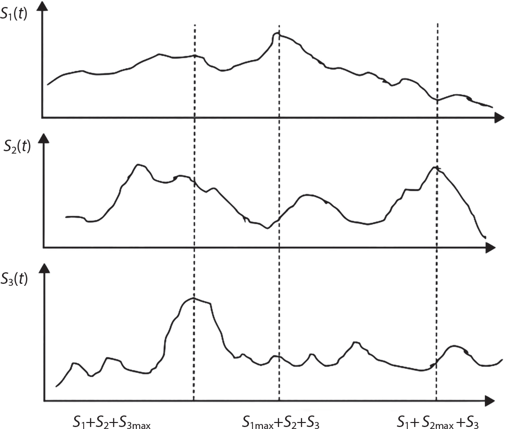
 be a positive whole number, and arrange it in increasing order of ri. So

 of xn(t, τn−1) and the density function fn−1(x) of xn−1(t). Therefore, the maximum value distribution can be determined by n-1 sequential convolution operations, as follows:

 , i.e.,
 represents the maximum value distribution of the i − 1th load effect in duration τi−1 of the ith load effect. The number of changes of Si in time interval τi−1 is
  . If pi = 1, then the distribution function of
  is
is  . The reliability index of structural components can be calculated by the PDF FMi(x) of the maximum load effect of various combinations according to the limit state concerned, and then taken as a minimum load effect combination, which is an optimal load combination for control structure design.
 represents the mean of the maximum distribution of the combined effect; μsi represents the mean of the truncated distribution of the effect of a single load. μsM varies with combination rules, while
  is only related to the inherent law of the loads involved in the combination, and is not affected by the combination method. The specific calculation results are as follows:
Load type
Mean (N/m2)
Coefficient of variation
Mean occurrence rate
Mean duration
Duration of time interval (Year)
Persistent live load
128.7
0.46
0.1
10 year
10
Temporary live load
48.8
0.69
1.0
0.01year
1
Wind load
66.67
0.45
1.0
10 minutes
1 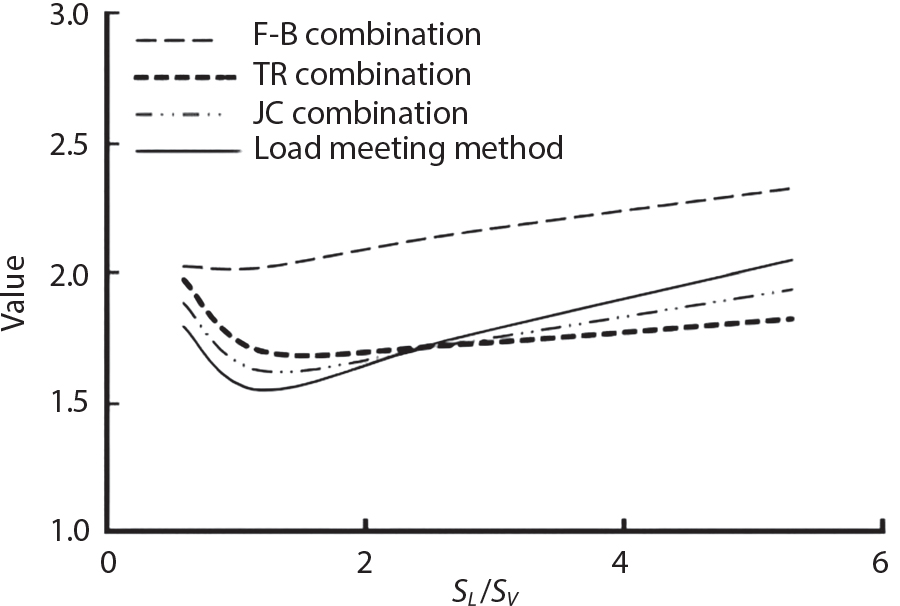
7.3 Calculation of Partial Coefficient of Structural Design
7.3.1 Expression of Design Partial Coefficient

 ,
, ,
, are design checking point coordinates for dead load, live load and resistance of structural components, respectively.
7.3.2 Determination of Partial Coefficient in Structural Design
7.3.3 Determination of Load/Resistance Partial Coefficient
 represents the standard value of resistance obtained by the probability method according to the target reliability index given the jth load-effect ratio of the ith structural component;
  represents the standard value of resistance obtained by the limit state equation based on the selected partial coefficient in the same situation, i.e.,
  .
.
 , thus enabling the error Hi to be minimized. The overall error I in the components and tubular joints of all common engineering structures is:
 values. Dimensionless relative error is used to achieve a balance in the ratio of the error of each component to the overall error.
 of structural component resistance, which changes with the load-effect ratio ρ, using the standard value
  of the structural component resistance determined by the design expression, given the target reliability index and dead load effect or live load effect. A linear function is used to fit it. If the error between the mean reliability index of components obtained by reverse calculation and the target reliability index is adopted for measurement, the effect is not so good when there are only a few optimization variables, but calculation is simple.
 is the target reliability index of the ith type of component; βij is the reliability index of the ith type of component in the limit state design expression at the jth ρ load effect ratio.
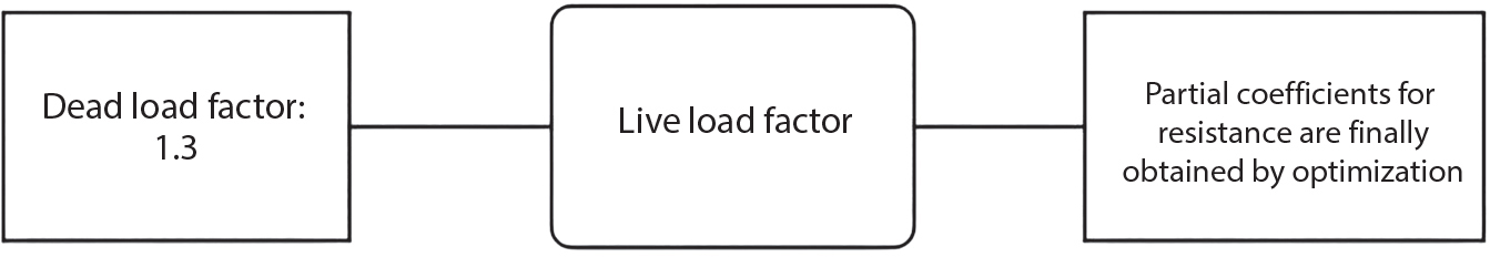
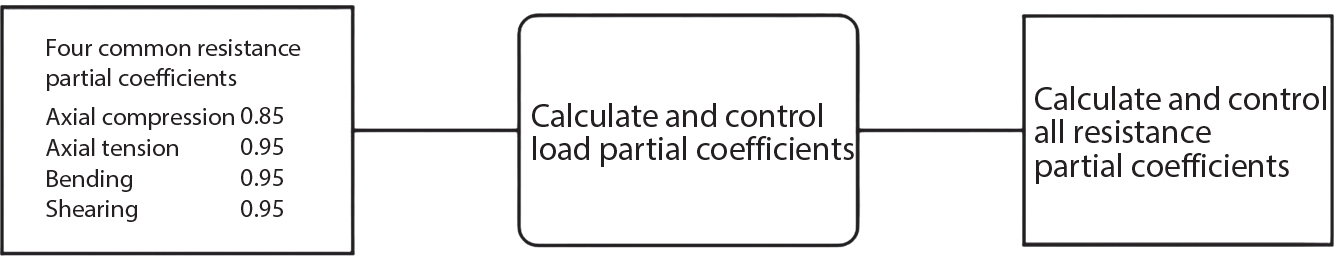
 , under the combination of dead load and live load. The calculation is as follows:
 can be calculated for each load combination, and each load-effect ratio ρ, and then substituted into the above equation to determine the resistance partial coefficients in the design expression under the condition that there is a minimum error between the designed reliability index of this structural component and the target reliability index.
7.4 Determination of Load Combination Coefficient and Design Expression
 of this variable load in the reference period is taken for probability limit state analysis. Given multiple variable load combinations, if the maximum distribution of each variable load in the reference period is still considered, this will become too conservative and unrealistic. The above-mentioned maximum distribution SM of load effect combination should be introduced into the limit state equation for probability analysis. This contains the maximum distribution of each variable load in a specific time interval. Theoretically, if the statistical parameters of these basic variables are known, then the resistance can be designed directly by the checking point method according to the target reliability index; or if the resistance is known, the reliability of the component can be checked when it is being acted upon by multiple variable loads. But at present, it is impractical to adopt probability design directly, while a partial coefficient design expression still needs to be presented in the codes for design value control [7-27][7-29]. Domestic and overseas design expressions considering load combination effect can be divided into the following two categories.
7.4.1 Design Expression Using Combined Value Coefficients

 represents the internal force caused by the standard value of live load (i.e., the standard value of load effect). When there are two or more short-term live loads applied, the
  of short-term live load should be multiplied by a combination coefficient of 0.9; m represents the number of live loads (including long-term and short-term live loads) acting at the same time; ni represents the coefficient of various loads, set to 1.2 for live floor loads and crane loads, 1.4∼1.6 for snow load, and 1.2∼1.3 for wind load; XG represents the internal force generated by the standard value of dead load, and the coefficient of dead load nG is set to 1.1, or to 0.9 when G is favorable.
7.4.2 No Reduction Factor in the Design Expression
 represents the effect caused by the mean value of dead load; LT,
 ,
, represent the effects caused by the mean value of the maximum distribution of live load, wind load and snow load throughout the service life;
  represents the effect caused by the mean value of the distribution of live load at any time point.
7.4.3 Method for Determining Load Combination Coefficient in Ocean Engineering

7.5 Example: Path Probability Model for the Durability of a Concrete Structure
7.5.1 Basic Concept
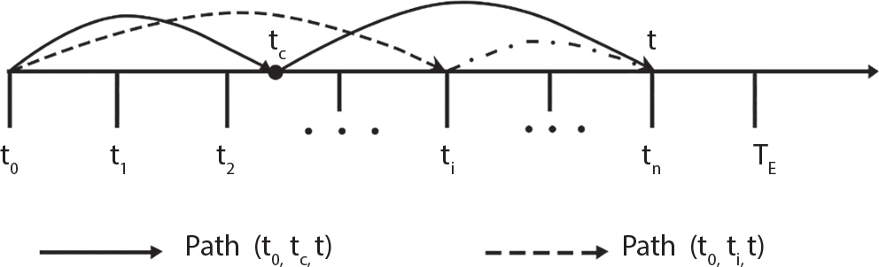
 which defines a possible corrosion path in
  . When TE has been determined, the corrosion ratio of any corrosion path
  is a function of time tc, and is recorded as
  ; η is the corrosion ratio of the steel bar.
 is further recorded as the probability density of the initial rusting of the steel bar at time tc, then the probability of initial rusting of the steel bar at time tc is
  . According to Bayes’ probability formula:
 is the conditional probability density function of the corrosion ratio of the steel bar under the condition that the initial corrosion occurs at time tc; a number of corrosion paths can be defined within
  .
.
 . then there are n corrosion paths
  ; these can contain all corrosion paths in
  , as long as n is large enough. When initial corrosion occurs at ti, then steel bar corrosion does not occur at any time before ti. Therefore, these paths are mutually exclusive. According to the probability summation formula, the unconditional probability density function
  of a steel bar corroding at time t can be expressed as:
 is the probability density function of the steel bar corroding under the condition that initial rusting occurs at time ti;
  is the probability of initial rusting of the steel at time ti,
 is the cumulative probability of initial rusting occurring at time ti.
7.5.2 Multipath Probability Model
 . It can be seen from the previous section that
  can be defined as many paths, and that any n time points in
  can be considered. For any initial rusting time ti(i = 1,2 … n) and protective layer cracking time
  , there are
  corrosion paths in total.
 , f(W) and f (L) for the corrosion ratio of steel bars, crack width due to corrosion expansion, and bearing capacity reduction coefficient in service time can all be calculated.
 and
and  are probability density functions of the crack width and bearing capacity reduction coefficient under the condition that ti and tk are determined, respectively;
  is the probability density function of protective layer cracking at time tk under the condition of initial rust occurring at time ti.
 should be considered. The time domain is divided into equal sections, with the time interval set as Δt;
  corrosion paths can thus be obtained, whose initial corrosion time, time of cracking due to corrosion expansion and late cracking time are all set as
 , there are altogether
  corrosion paths, whose initial corrosion time, time of cracking due to corrosion expansion and late cracking time are all set as
 can be derived from the path defined by the maximum service time, and only the paths defined by
  need to be simulated.
7.5.3 Probability Prediction Model Featuring Chloride Erosion
 is the chloride ion concentration (percentage of concrete mass) at a distance x from the concrete surface kg / m3; C0 is the concentration of initial chloride ion inside the concrete (usually 0); Cs is the concentration of chloride ion on the concrete’s surface, Val [7-43] considers that its distribution parameters are related to the environment, and it is recommended to take values based on Table 7.3; Dcl is the chloride ion diffusion coefficient mm / s. Stewart believes this is related to time, temperature, humidity and stress level, and assuming a condition of no measured data, it can approximately obey a normal logarithmic distribution with a Mean Value of 2×10⁻⁶ and a coefficient of variation of 0.450 [7-44];
Environment types
Mean
Coefficient of variation
Distribution types
Splash areas
7.35kg/m3
0.70
Log-normal distribution
Near-shore environment
2.95 kg/m3
0.70
Log-normal distribution
1km from coast
1.15 kg/m3
0.50
Log-normal distribution
Normal atmospheric environment
0.03 kg/m3
0.50
Log-normal distribution
 of initial rusting of the steel bar occurring at any time ti can be expressed as:
7.5.4 Probability Prediction Model for Concrete Carbonation
Concrete strength grade
C15
C20
C25
C30
C35
C40
C45
C50
C55
C60
Standard value/MPa
22.86
28.33
33.75
39.29
21.54
50.00
55.83
60.91
67.27
72.00
Coefficient of variation
0.21
0.18
0.16
0.14
0.13
0.12
0.12
0.11
0.11
0.10 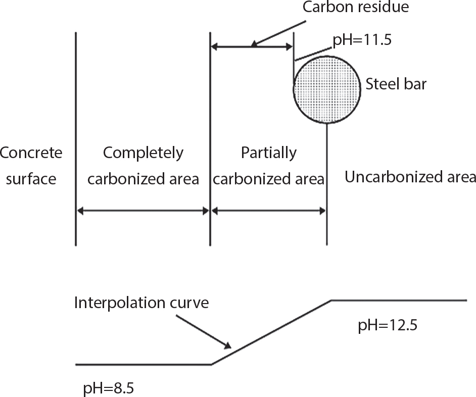
 of initial rusting occurring in a concrete steel bar at any time ti can be expressed as:
 is the length of the complete carbonation zone at the point of initial rusting of the steel bar (mm).
7.5.5 Probability Prediction Model under the Combined Action of Carbonation and Chloride Ions
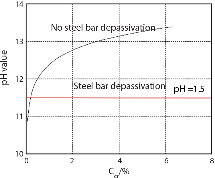
 can be expressed as:
7.5.6 Corrosion Propagation in a Steel Bar
 . The specific calculation process can be expressed as:
 , Xc is the thickness of the concrete protective layer (mm),
  is the standard value of the compressive strength of the concrete cylinder MPa [7-51], [7-52], and fc is the standard value of the compressive strength of the concrete cube (MPa).
7.5.7 Cracking of the Protective Layer and Determination of Crack Width
7.5.8 Bearing Capacity of Corroded Concrete Components
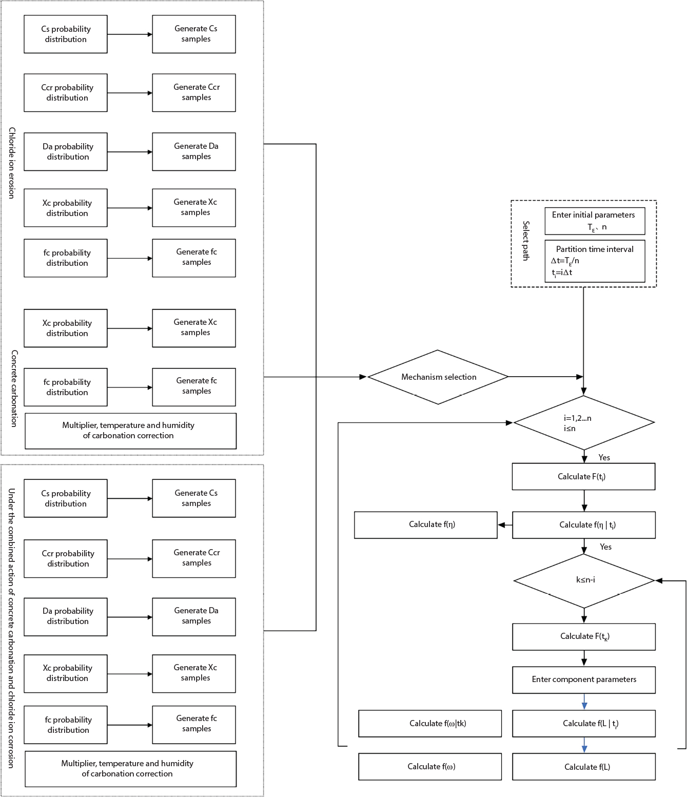
7.5.9 Engineering Example
7.5.9.1 Corrosion of Steel Bars in a Chloride Environment
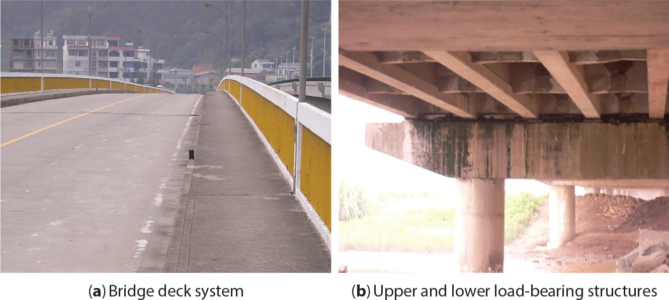
Parameter type
Unit
Mean
Coefficient of variation
Distribution type
Source
Cs
kg/m3
7.35
0.7
Logarithmic normal
Stewart[7-8]
Dcl
mm2·s-1
2×10⁻⁶
0.45
Logarithmic normal
Stewart[7-8]
Xc
mm
35.2/29.8
0.060/0.066
Logarithmic normal
Measured value
Ccr
kg/m3
3.35
0.375
Logarithmic normal
Stewart[7-8]
fc
MPa
29.9
0.064
Logarithmic normal
Measured value
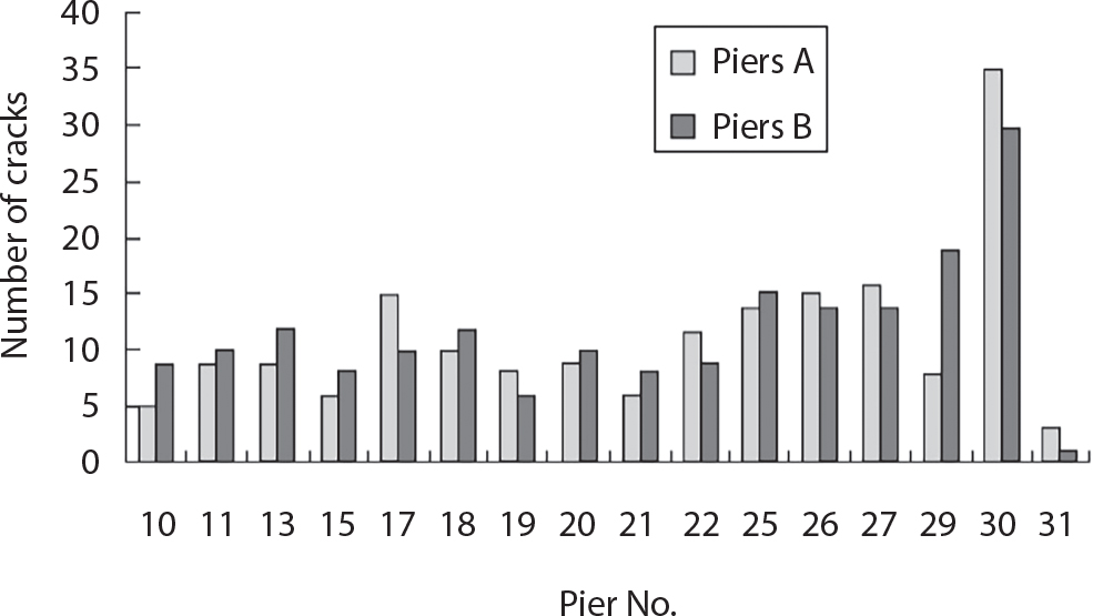
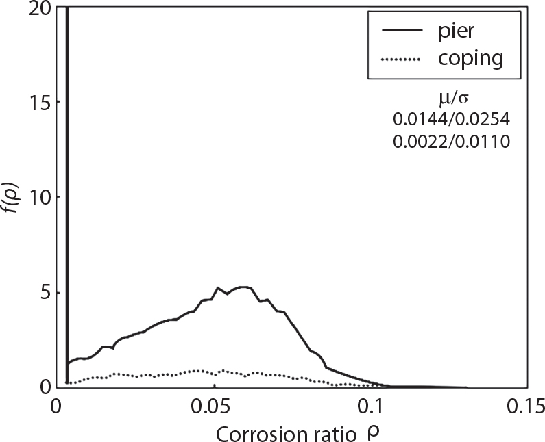
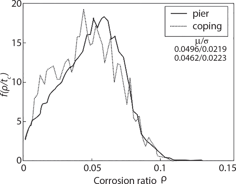
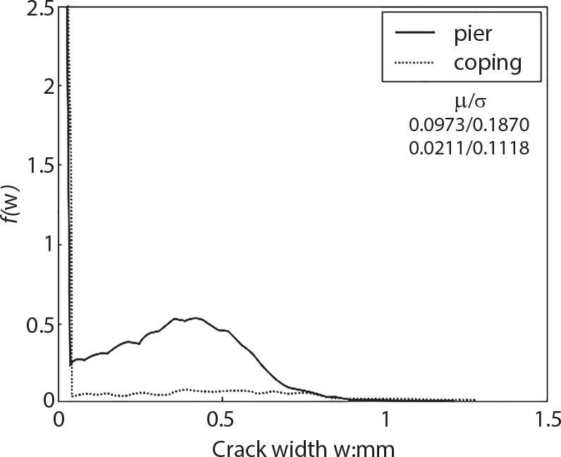
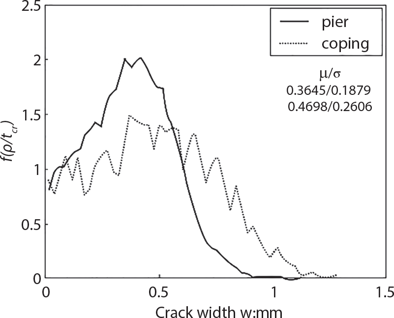
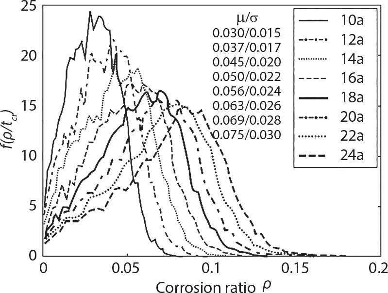
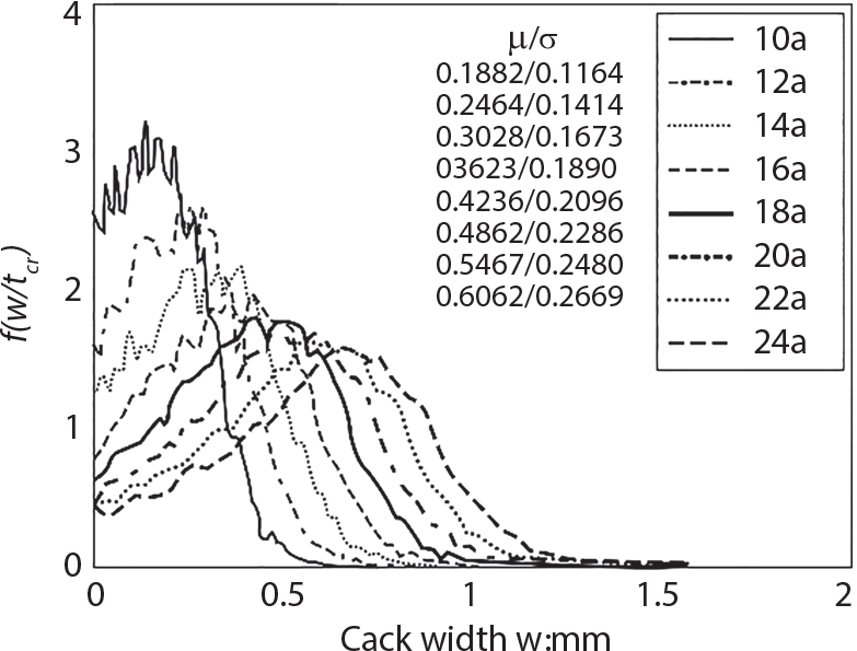
7.5.9.2 Corrosion of Steel Bar Under the Combined Action of Carbonation and Chloride Corrosion
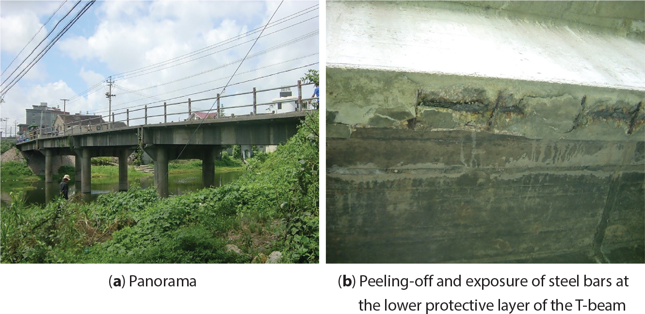
Parameter type
Unit
Mean
Coefficient of variation
Distribution type
Sources
Cs
kg/m3
2.95
0.7
Logarithmic normal
Stewart[7-8]
Dcl
mm2·s-1
0.167×10⁻⁶
0.45
Logarithmic normal
Measured value
Xc
mm
15
–
Constant
Measured value
Ccr
kg/m3
3.35
0.375
Logarithmic normal
Figure 7.15
ds
mm
2Φ20
–
Constant
Design value
dv
mm
Φ6@ 200
–
Constant
Design value
fy
MPa
365
0.05
Logarithmic normal
Design value
fc
MPa
25
0.15
Logarithmic normal
Measured value
T
°C
20
–
Constant
Meteorological survey
RH
%
75
–
Constant
Meteorological survey

%
0.03
–
Constant
Meteorological survey

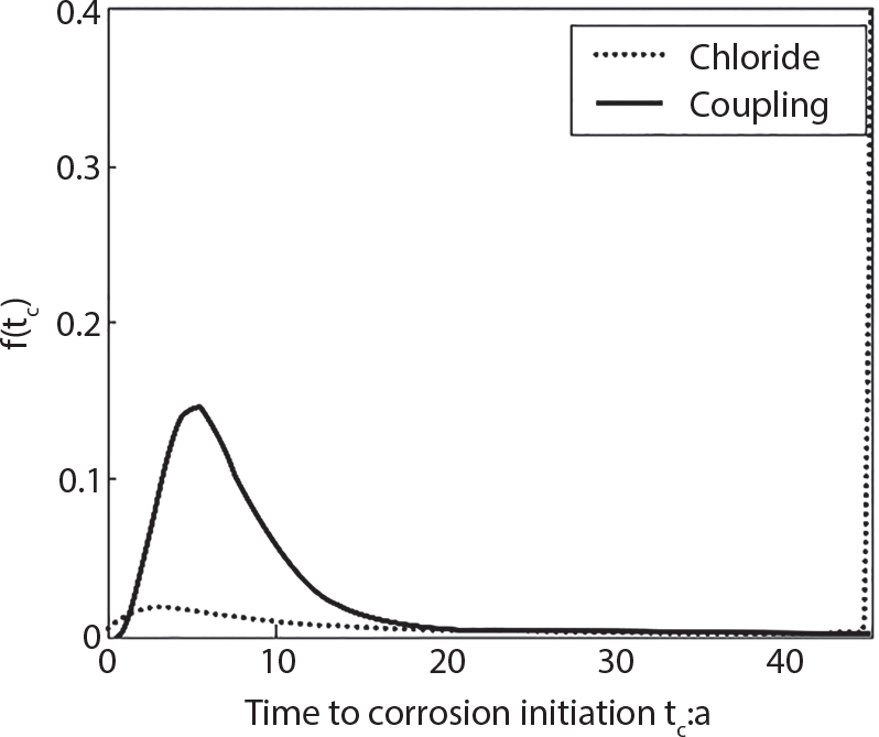
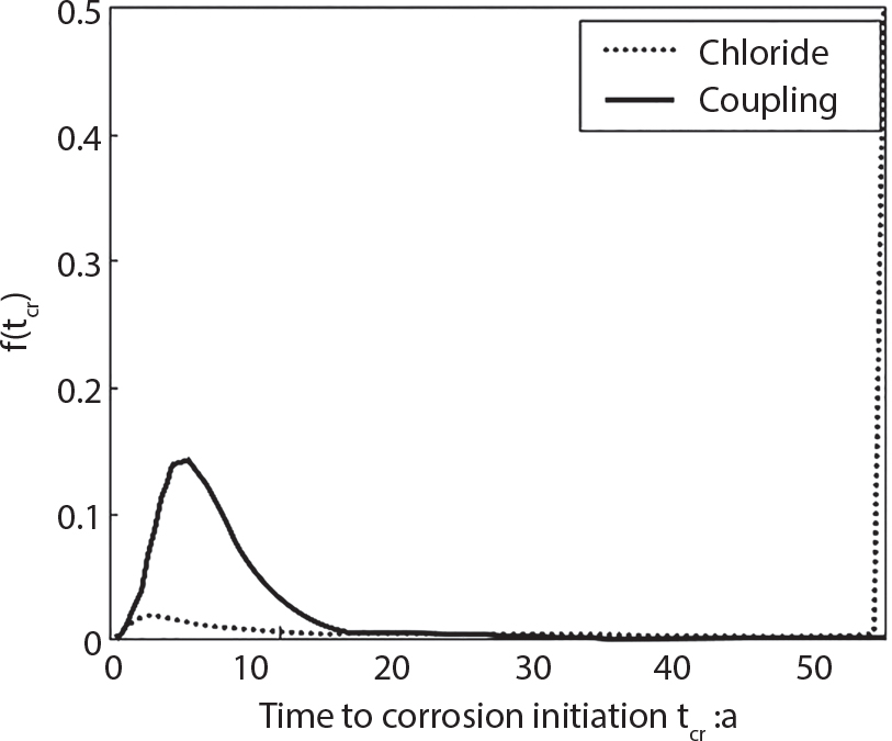
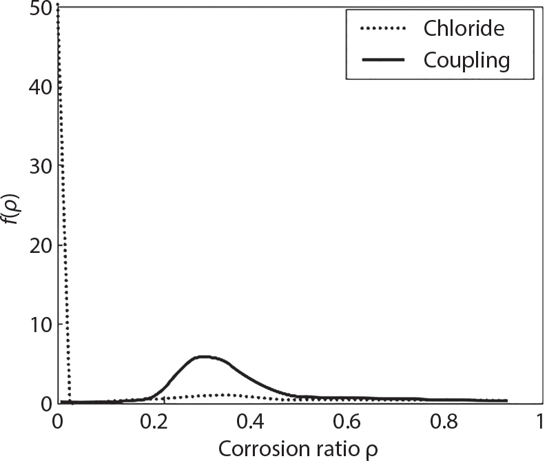
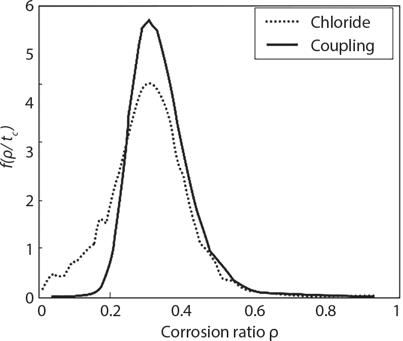
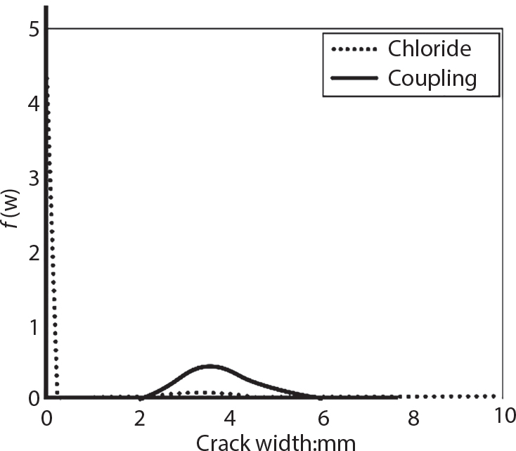
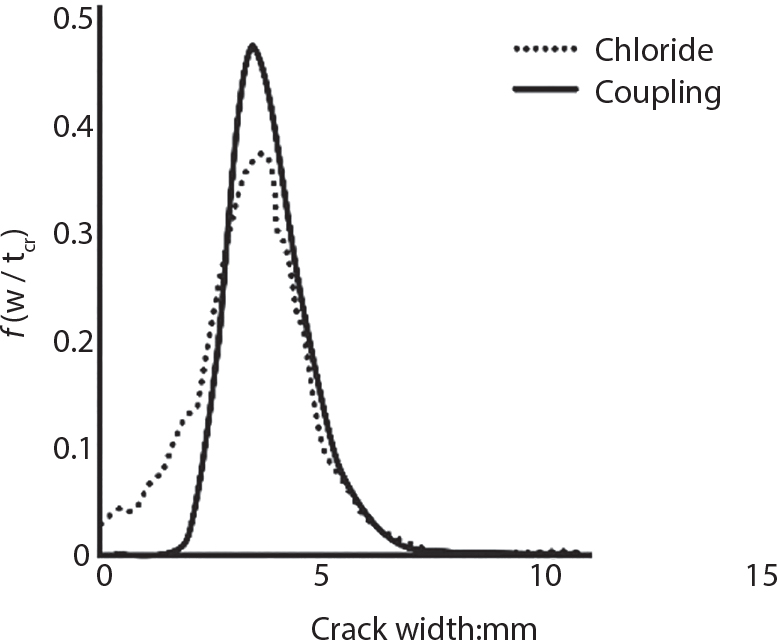
References