The problem of structural reliability is one of dealing with the uncertainty of things. If there is an inevitable causal relationship between the conditions for the occurrence of an event and the results of such an occurrence, then the event can be called a definite phenomenon. Likewise, if there is no inevitable causal relationship between the conditions for the occurrence of an event and the results of the event, then such an event is known as an indefinite phenomenon [2-1]. In fact, there are many indefinite phenomena in nature and engineering practice. In the analysis and application of structural reliability, the reliability of a structure is affected by both subjective and objective factors. For example, objective factors involved in engineering structure design include random variables such as action, environmental effects, materials and geometric parameters. In the process of engineering decision-making, people often make use of structural reliability analysis tools, thereby bringing about subjective uncertainty. Artificial level of understanding should be taken into consideration, and it is also necessary to clarify the impact of subjective uncertainty on reliability analysis and predictions. As a matter of fact, the comprehensive effect of various uncertainties should be considered with respect to structural reliability analysis, design, evaluation and prediction[2-2], especially when the reliability of an existing structure is being assessed[2-3]. It should be noted that as people deepen their understanding of the objective world, a variety of methods are constantly emerging to handle uncertainty, making it possible to analyze the uncertainties of structural reliability in a more comprehensive way[2-4]. The uncertainty, in terms of its types, characteristics, forms and attributes, introduces uncertainty classification methods, and sets forth methods for uncertainty analysis are classified in this chapter. These methods include the probability analysis method, fuzzy mathematics method, gray theory method, relative information entropy analysis method and artificial intelligence (AI) analysis method. In nature and engineering practice, there exist many indefinite phenomena. For example, during structural design, it is impossible to know exactly the required size of a structure that can help effectively resist wave load, wind load and snow load. Neither is it possible to know exactly whether the material characteristics of such a structure are unique. In short, the uncertainty means that the occurrence or result of an event is uncertain, or that the result cannot be foreseen before the occurrence of the event. This is mainly manifested as follows: (1) the upper limit of various structures and loads, as well as the lower limit of material strength are actually difficult to define; (2) even if there is such a natural limit, it is likely to be very uneconomical in practical applications (extreme load); (3) the limit imposed by quality control and testing is not completely effective, while a change may take place in the potential performance; and (4) even if there is an accepted limit, its use is not always necessarily reasonable (maximum load, minimum resistance). Due to the difference in research object and solution, the problems of structural uncertainty can be expressed by the following classification methods. (1) Aleatory uncertainty Aleatory uncertainty represents the intrinsic, inherent and fundamental uncertainty of basic variables. It refers to the natural randomness of physical quantities and cannot be eliminated. Aleatory uncertainty is a type of objective uncertainty, which is determined by internal factors and external conditions, such as the uncertainty of load, material properties and geometric dimensions. (2) Epistemic uncertainty Epistemic uncertainty is a type of uncertainty arising from limited information and understanding. It can be further divided into statistical uncertainty, model uncertainty and measurement uncertainty. The first is caused by limited observations and depends on the sum of sample data and any existing knowledge; model uncertainty is caused by the defects and idealization of the physical model; measurement uncertainty is caused by the inaccuracy of the methods and tools used to evaluate a variable. Generally, knowledge uncertainty can be reduced by collecting more information in a more careful manner, or by adopting a more sophisticated model. (1) Objective uncertainty Objective uncertainty refers to all countable information from an event. It is random and can be described mathematically, involving only variables. (2) Subjective uncertainty Subjective uncertainty refers to all uncountable information from an event, caused by human activities. It is characterized by fuzziness, ignorance and incomplete knowledge. Often expressed by the Fuzzy theory, it involves not only variables, but also system processes. (1) Random uncertainty The concept of random uncertainty means that the result of an event is uncertain because the conditions for its occurrence are out of control, but the result still has a clearly defined range of variation. Random uncertainty (called randomness for short) boasts a certain category of items, and the concept of randomness has a certain extension, but its connotation is uncertain. It can be expressed by a mathematical expression. For example, variable uncertainty obeys normal distribution. In general, the reliability uncertainty analysis method, which is a probability method, can be used. (2) Fuzzy uncertainty Fuzzy uncertainty (called fuzziness for short) is caused by the boundary uncertainty of variables, characterized by “fuzziness”. Fuzzy things fall under an uncertain category. The concept of fuzziness has a clear connotation, but its extension is unclear. It is usually described in fuzzy words. From a philosophical point of view, fuzzy uncertainty is a higher form of random uncertainty. In general, the fuzzy random structural reliability theory based on fuzzy set theory can be used. (3) Incompleteness Incompleteness is caused by a lack of knowledge. Its concept has a clear yet unclear connotation, i.e., “some information is known, whereas some is unknown”. Normally, it can be described by means of the gray theory, by the neural network theory and turbidity, and by the bifurcation theory. In general, reliability uncertainty analysis methods, such as gray theory and information theory, can be adopted. (1) Parameter uncertainty[2-5] Parameter uncertainty is caused by the uncertain knowledge of basic variables or events. As a fuzzy random problem, it arises from the randomness, fuzziness and incompleteness of variables. (2) System uncertainty [2-5] System uncertainty is caused by the inadequacy of the theoretical model or failure probability. It is the rest (in the sense of remainder) of parameter uncertainty. It is primarily caused by human activities and incompleteness. If the joint probability density function f(x) of random variables of a structure is known, then the failure probability Pf of the structure can be expressed as: where Df represents the structural failure zone. This kind of method is commonly used in the traditional structural reliability method based on the probability characteristics of variables[2-6]. Subjective judgment is completely ruled out because objective probability is adopted as part of classical probability theory and reliability is calculated based strictly on assumed objective distribution. It is usually very difficult to establish a total probability distribution function. In general, the first and second moments of distribution parameters are used to approximately describe the uncertainty of basic variables. Subjective judgment is expressed by the rule of objective probability. The new formula obtained from conditional probability is as follows: where P(Ai) represents prior probability; B can be regarded as a proposition supported by the new experimental results. P(AiB) represents revised prior probability; in this way, it can not only combine objective events together, but also combine objective probability with subjective judgment, greatly broadening the application scope of the probability theory. However, one of the premises of Bayes probability is: When P(A) is used to express the degree of artificial subjective belief in proposition A, a conclusion can be drawn, as follows In other words, human cognition is only composed of certainty A and uncertainty Fuzzy mathematical analysis is primarily used to solve uncertainty problems with an inexact definition and unclear boundaries. Zedeh[2-7] was the first person to introduce the concept of fuzzy subsets into the idea that basic variables are not taken as deterministic values or stochastic variables, but rather represented by discrete feature points. This means that the fuzzy subset A can be represented as where μA(X) is the membership function of A; x ∈ U is a universe of discourse, 0 ≤ μA(X) ≤ 1, x → μA(X). The above formula is called Zedeh notation, and is not a sum formula. If μA(X) is a continuous function, then the Zedeh notation is The rest of the fuzzy subset A is denoted as Union A ∪ B = C ⇔ for ∀ x ∈ U x ∈U, so Intersection A ∩ B = D ⇔ For x∀∈U, so The common representations of a membership function are as follows in Table 2.1: In where, if [L] = μL, then Table 2.1 Representation of membership function. The subjective uncertainty of a basic variable A can be expressed by the following steps. Let subjective uncertainty be Ei. The measurement criteria are as follows: (i) Mi is the level of Ei; (ii) Gi is the importance of Ei. So For all subjective uncertainties, there is There should be a fuzzy conditional relationship between M and A Therefore, the fuzzy relationship between subjective uncertainty and basic variable A is as follows This means the membership function derived from the importance of subjective uncertainty is as follows Accordingly For this method, the key is how to determine the membership function μA(X) of the basic variable A. The gray theory[2-8] can be used to study an uncertainty problem featuring a small sample size and insufficient information. The gray system (G system) is a semi-open and semi-closed system for a certain level of understanding, where some information is known while the rest is unknown, i.e., the information is incomplete. A system containing completely clear information is called a white system; a system containing unknown information is called a black system; a system containing some clear information and some unclear information is called a gray system. System information incompleteness is divided into four types: (1) incomplete element information; (2) incomplete structural information; (3) incomplete boundary information; and (4) incomplete information on operating behavior. The gray theory is characterized by information incompleteness and the non-uniqueness of results obtained. Therefore, theories have been devised including the principle of information incompleteness and the principle of process non-uniqueness. The solving process for non-uniqueness is a combination of qualitative and quantitative analyses. By supplementing information, qualitative analysis can be used to determine one or several satisfactory solutions. That is how the gray system is solved. System information incompleteness is divided into four types: (1) incomplete element information; (2) incomplete structural information; (3) incomplete boundary information; and (4) incomplete information on operating behavior. If the connotation and extension of an object are completely certain, it is white; if it has an uncertain connotation and a certain extension, it is gray; if it has a certain connotation and an uncertain extension, it is fuzzy; if both connotation and extension are uncertain, it is gray fuzzy. For the basic variable z, its value changes at interval h, making it a gray variable, denoted by ⊗(z). or expressed in discrete form, ⊗(z) = {hi, i ∈ I, hi, ∈ R}; different coefficients on ⊗(z) are expressed in fGray(z), where fGray(z) is the built-in function of ⊗(z), or its whitening weight function [fGray(z) ∈ (0, 1)]. The whitening weight function has the following attributes: Expressed in discrete form, For the carbonized depth in concrete[2-9], this can be represented by a gray area, and a region can be set for β. where i = 0, 1, 2, ……, N, N +1. A is the factor of carbon velocity. B is a parameter of concrete carbonization, is about 0.4 to 0.6. Given the concrete carbonization qualification index do, the failure probability of concrete carbonation durability Pf = P(do ≤ d) and Table 2.2 Digital representation of gray scale. Because the corresponding carbonized depth in concrete is a weighted interval number at time t, β also has a weighted average. The specific calculation process is as follows: The weight where i = 0, 1, 2, ……, N, N +1. where i = 0, 1, 2, ……, N, N +1 According to the relative information entropy theory and the definition of parameter and system uncertainty, the objective uncertainty of a basic variable X can be represented by the Shannon entropy[2-10] where p(xi) represents the distribution probability of the ith discrete point of variable xi. If the subjectivity π(xi/R) of parameter uncertainty comes mostly from that of the probability distribution of variable xi and that of the variable distribution interval caused by R, then the subjectivity can be represented by a relative information ambiguity function, while its relative information entropy[2-11] can be described by means of Equation (2.22) Considering that the limit state function z=g(X) is a function of basic variables and xi is a relatively fuzzy variable with parameter uncertainty, let The right end of the equation can be obtained from the combination rule Equation (2.23) of relative information. Hence, the relative information entropy of the structure caused by parameter uncertainty can be written as: where superscript P represents parameter uncertainty and H(Z) is the Shannon entropy of probabilistic reliability analysis. So where Pf represents the probability of structural failure revealed by probabilistic reliability analysis. The impact of system uncertainty is taken into consideration to build a relative information ambiguity function for system uncertainty. Therefore, the total relative information ambiguity function of parameter and system uncertainties can be obtained from Equation (2.26) Similar to Equation (2.25), the relative information entropy of the structure is as follows The Shannon entropy method is used to represent the impact of parameter uncertainty and system uncertainty in order to compare with the results of probabilistic reliability analysis, i.e., An ANN (Artificial Neural Network) is a theoretical mathematical model of the human brain and its activities. Composed of a great many processing units properly interconnected, an ANN is a large-scale nonlinear adaptive system[2-14]. Featuring excellent nonlinear mapping and associative memory capabilities, ANNs are widely used for function fitting under various complex relations, and show both great flexibility and good adaptability. ANNs helps to provide more accurate calculation results without the aid of explicit mathematical and physical models. Moreover, they can boast good fault tolerance and adaptability. These characteristics make ANNs suitable for the time-variant reliability evaluation of structures. Among neural network algorithms, the most widely used is a multi-layered feed forward neural network based on error back propagation, the BP (Back Propagation) neural network. The BP learning algorithm is adopted in the BP neural network, which is composed of both forward propagation and back propagation. Forward propagation means transmitting the input signal from the input layer to the output layer via the hidden layer. If the signal is properly output from the output layer, the learning algorithm will end; otherwise, back propagation will be enabled. Back propagation involves reversely calculating the error signal (the difference between sample output and network output) along the original connection route, with the gradient-descent algorithm used to adjust the weight and threshold of neurons in each layer to reduce the 4error signal. BP is a widely used neural network characterized by high operability, low computational complexity and low parallelism. Structurally, the BP neural network consists of an input layer, an output layer and one or more hidden layers. The neural network is a process of mapping from the input surface to the output surface. This type of mapping is realized by means of the transfer function. There are two kinds of transfer functions commonly used in the BP neural network: purelin and sigmoid. Sigmoid functions include the symmetric tansig function and the asymmetric logsig function. See Figure 2.1. If there are enough elements in the hidden layer, two layers can approximate any continuous function. Figure 2.2 shows a typical BP neural network containing two hidden layers. P represents the input parameter; IWi represents the set of weights in the i-th layer; F1 and F2 are transfer functions tansig and purelin in the first and second hidden layers, respectively; a1 is the intermediate variable generated after the input parameter is transmitted through the first hidden layer, and also the input parameter of the second hidden layer; the output parameter a2 is obtained after a1 is transmitted through the second hidden layer. Figure 2.1 Three types of transfer function. Figure 2.2 Diagram of two-layer BP neural netbook structures. The following is the specific process by which the BP responding surface method is used for structural reliability analysis: SVM (Support Vector Machine) is a general machine learning method based on the statistical learning theory. Its idea originated from the support vector method proposed by Vapnik et al.[2-15] in 1963 to solve the pattern recognition problem. SVM maps the original space of the problem to a higher-dimensional feature space, where the classification problem can then be solved. When the classification problem is solved, it is considered that only the vectors on the classification boundary play a role in classification; these vectors are called support vectors. In Figure 2.3, a, b, c, d and e are support vectors. This is where the method gets its name. The principle of structural risk minimization is applied to SVM, enhancing the generalization ability of the learning machine. This means that a small error is still bound to be generated even if a solution is obtained from limited training samples. There is a strict theoretical basis for SVM, capable of solving practical problems featuring a small sample size, nonlinearity, high number of dimensions and a local minimum. Considering this, the implicit limit state equation can be reconstructed in a new manner for structural reliability analysis. For response surface reconstruction by SVM, it is essentially a process of building a regression support vector machine (RSM)[2-16]. For SVM, regression is the same as pattern recognition, because it is also a process of mapping the input vectors in the original space to a higher-dimensional feature space, where a classification problem is taken into consideration. The mapping from the original space to a higher-dimensional feature space is realized by using the inner product in the feature space described by the kernel that meets the Mercer condition. Figure 2.4 shows the basic process of how RSM is implemented. Figure 2.3 Diagram of support vectors. Figure 2.4 Diagram of regression support vector machine. (1) SVM response surface reconstruction A quantitative method that makes a trade-off between approximation precision and approximate function complexity for a given set of sample data is adopted for RSM. A set of feature subsets is selected from the training set so that the linear division of the feature subsets are equivalent to the segmentation of the entire dataset. For RSM in linear loss functions, the following optimization problem needs to be solved where vector w and scalar b control the position of the optimal classification plane; (xi, yi) is a training point set; C is a penalty function, reflecting the coordination between structural and empirical risk; ε is the error insensitivity coefficient; ξ and ξ* are slack variables. Under Kuhn-Trucker conditions, Equation (2.30) is transformed into the following dual problem: where α* and α are Lagrange multipliers; l represents the number of support vectors. Equation (2.31) is a convex set programming problem and has a unique solution. In other words, there is an obvious theoretical basis for the determination of the network topology of SVM. This is also one of its advantages over neural networks. The complexity of the process of solving Equation (2.31) is determined by the number of samples with a nonzero weight, i.e., the support vectors. During the development of its solving algorithms, SMO (Sequential Minimal Optimization) [2-17] was gradually developed on the basis of the Chunking and Osuna algorithms. SMO can decompose a large-scale QP (Quadratic Programming) problem into a series of smaller QP problems containing 2 Lagrange multipliers only, making it possible to solve the primal problem by a semi-analytical method. After Equation (2.31) is solved, the optimal regression function of RSM is as follows: The training point set in Equation (2.32) is composed of the empirical points corresponding to the input and the response obtained by the structural finite element method. It is the structural limit state equation reconstructed by SVM. Different kernel functions can be used to obtain different response surface equations. Commonly used kernel functions include linear kernel, polynomial kernel, RBF (radial basis function, or Gaussian) kernel and two-layer neural network kernel. However, there is no satisfactory method for choosing an appropriate kernel function, meaning they need to be selected based on experience. (2) Deduction of partial derivative for SVM regression function The FORM/SORM for reliability calculation requires the use of a partial derivative of the limit state equation. A first-order partial derivative is required if FORM method is used for calculation. For the reconstruction of the response surface Equation (2.32), let support vector (i) Linear kernel Kernel function Its response surface function In which b is a constant, so (ii) Polynomial kernel Kernel function Its response surface function so where d represents the order of the polynomials. (iii) RBF kernel Kernel function Its response surface function so where γi is a constant, which determines the width of the function around the center point. (iv) Sigmoid kernel Its response surface function so Where v(X·Xi)is a linear kernel, but S[•] is function of v(X · Xi). c and b is a constant, respectively. (3) Calculation steps for SVM-based responding surface method The traditional responding surface method for structural reliability analysis consists of two processes: the reconstruction of a local response surface near the expansion point and the search for the design point. For the SVM-based responding surface method, SVM is used to reconstruct the response surface, while the geometric reliability method is used to calculate the design point and structural reliability. The steps are as follows: A 10-storey beamless floor structure with a storey height of 3m, column grid size 6,000mm×6,000mm, column size 550mm×550mm, and slab thickness of 200 mm; concrete strength of the concrete slab and column: C30; reinforcement in positive and negative moment field: HPB235 steel and HRB335 steel. Area of reinforcement at support: 1,214 mm2/m; area of reinforcement at midspan: 808 mm2/m. Fastener-type steel pipe formwork is used for support. Steel pipe φ48 mm×3.5 mm; vertical rod spacing 750 mm; step distance 1,700 mm. Section stiffness of the bracing system is 6.4×10³ kN, determined after considering the influence of wood keel on bracing stiffness and the depreciation effect of steel uprights. In particular, the length is calculated together with the stable bearing capacity of the formwork support system, according to the code. Where, h is the step distance, a is the length of the rod extending from the top cross bar of the formwork. In this example, a is 0. The maximum value calculated by the code is taken as the stable bearing capacity of the formwork. When the stability coefficient is calculated using the Monte-Carlo method, if the length calculation coefficient μj < 1.0, then μj is taken to be 1. In order to evaluate the construction risk of fastener-type steel pipe formwork, it is necessary to first establish a risk evaluation system. The construction safety of the fastener-type steel pipe formwork is affected by a variety of factors, which can generally be divided into two categories, the first of which is on-site construction. Throughout the entire process, from scaffold design to dismantling, each link directly affects formwork safety. The second category is safety management, which must be underlined throughout the whole construction process, and which exerts a significant influence on formwork safety. Both of these can be further divided into sub-indices. Scaffold collapse is the main type of safety accident that occurs, with every link in the formwork erection process affecting safety. Design scheme, materials and erection, inspection and acceptance, and loading and dismantling all fall under key influential indices, so the construction indices are divided into these six aspects. Safety management and site construction are closely related and interact with each other. Effective auxiliary safety management is entailed in the whole formwork construction process. A multi-index and multi-level risk evaluation system[2-18] was duly established based on the above analysis, and after soliciting advice from numerous design and construction experts for fastener-type steel pipe formwork. Table 2.3 Indices and weights of a risk evaluation system for fastener-type steel pipe formwork support construction. The evaluation system includes a total of five levels: Table 2.3 shows indices and weights of a risk evaluation system for fastener-type steel pipe formwork support construction. In the evaluation system shown in Table 2.3, the importance of each index varies, making it necessary to determine the weighting of each index. This index weighting can be determined by such methods as the Analytic Hierarchy Process (AHP) [2-19], expert scoring method, or others. To be specific, an expert scoring method is adopted to determine the appropriate weighting by means of a questionnaire, the respondents to which are construction site managers. To reflect the influence of the respondents’ educational background μ1, age μ2, working years μ3, and safety education μ4 on the weighting judgment, the questionnaire also contains some questions regarding these aspects. Table 2.4 Rating scale table. The importance of the indices in the questionnaire is further divided into 10 grades, from 1 (no influence) to 10 (most important). See Table 2.4 for details of this classification. A total of 84 questionnaires were collected for the 10 projects investigated. The calculation formula for the importance of each index can be expressed as: Relative weighting of the indices can be expressed as: Where, μi1, μi2, μi3 and μi4 represent the weighting of educational background, age, working years and safety education, respectively. Their values are determined as shown in Table 2.5; Ri is the specific score of indices in a single questionnaire received. See Table 2.4 for the scoring standard; n is the number of questionnaires collected; Si is the importance of each index in the same level index; Wi is the relative weight of each index in the same level index. See Table 2.5 for the importance and relative weights of each index after processing. Table 2.5 Weighting of individual differences. The score value x(x ∈ [0,10]) of each evaluation index indicates the actual implementation status. Questionnaires were distributed to managers, who were required to score all grades of the indices according to the realities on site, in order to determine the score for each index. A total of 120 questionnaires were collected from the 10 projects investigated. Respondents were asked to evaluate the risk of formwork construction in the industry using a 10-point system. See Table 2.6 for the averaged results of the experts’ scores. Uncertainties in the scoring of various evaluation indices of the formwork support system are inevitable, since they reflect the inherent features of the framework support system. When using random statistical methods, only the random uncertainty of the index score value can be considered, not its own fuzzy uncertainty. Therefore, the score value of each index was fuzzed, as shown in Figure 2.5. In Figure 2.5, the score was Table 2.6 Expert ratings. Figure 2.5 Fuzzineation of score values. Where, the value of c reflects the fuzzy boundary range of random variables, which is determined according to project realities; in general, According to the realities of construction risk evaluation for fastenertype steel pipe formwork, the evaluation grade was divided into five grades. V={v1, v2, v3, v4, v5}={Grade 1, Grade 2, Grade 3, Grade 4, Grade 5}={Least safe, unsafe, relatively safe, safe, and safest}, represented by a fuzzy function in Figure 2.6. Figure 2.6 Membership function of the evaluation grade. Taking the actual data collected as an example, the fuzzy grey correlation method and the traditional multilevel grey correlation analysis method were used, respectively, to describe the step-by-step data flow process in the risk evaluation system for formwork construction, and to explain the calculation method of multi-index multilevel grey correlation analysis. Superscript (1), (2) and (3) in the following table (Table 2.7 and Table 2.8) show the calculation results for the fuzzy grey correlation analysis method as represented by plane distance, lattice distance, and traditional multilevel grey correlation analysis, respectively. Table 2.7 Correlation matrix for each index in the D-layer; relative weight and correlation coefficient matrix of fastener and pole index. Then the correlation matrix for the fastener installation indices D10 The correlation matrix for the vertical rod indices D11 Table 2.8 Relative weighting and correlation coefficient matrix of materials and erection indices. 2) Correlation degree matrix for each index in level C Then the correlation matrix for the material index C7 The correlation degree matrix for the erection index C9 The calculation for dismantling and load index is the same as above. 3) Calculation of correlation degree matrix for each index in Level B The calculation method is the same as that for Level C and Level D, so the detailed calculation process can be omitted. The result is shown in Table 2.9. Correlation degree matrix for safety management index B1 Correlation degree matrix of field construction index B2 Table 2.9 Relative weight and correlation matrix of index. 4) Calculation of correlation degree matrix for each index in Level A The correlation degree matrix for construction risk of a fastener-type steel pipe formwork can be expressed as: 5) Determining the construction risk of fastener-type steel pipe formwork The correlation degree is a numerical representation of the close relationship between sequences. When studying the correlation between reference sequences and compared sequences of a system, special attention should be paid to the order of the correlation degree between reference sequences and compared sequences, that is, the ranking of the correlation degree, rather than the magnitude of the correlation degree in numerical terms[2-21]. According to the principle of maximum correlation degree identification, the results of the three methods are consistent, and the construction risk grade for fastener-type steel pipe formwork investigated on site is Grade 4, which falls within the safety scope. The ranking for the correlation degree obtained by the first two methods where fuzziness is considered is completely consistent, but slightly different from that obtained by the traditional method of multilevel grey correlation analysis. In the former two methods, where the fuzzification of standard index values and score values are considered, the ranking of the correlation degree better complies with the objective requirements. In this paper, fuzzy numbers were introduced into grey relational multilevel and multi-index analysis theory, and a grey comprehensive evaluation method based on fuzzy numbers was proposed. The distance of the fuzzy numbers is represented by plane distance and grid distance. Regarding the standard index value and the index score value as fuzzy numbers enables the complexity and inherent fuzzy uncertainty of objective items to be considered more easily, thus making multilevel grey correlation analysis more scientific and bringing it closer to reality. This method is applied to the construction risk evaluation of fastener-type steel pipe formwork. The results show that the grey correlation ranking obtained via the improved grey correlation analysis method (based on two fuzzy number distances) is completely consistent, but slightly different from the traditional grey correlation analysis method. This method can facilitate the comprehensive quantitative evaluation of fastener-type steel pipe formwork safety, avoid subjective randomness during risk evaluation, and help managers understand and master site safety in a timely manner, thus improving enterprises’ ability to carry out proper accident control.
2
Method of Uncertainty Analysis
2.1 Classification of Uncertainty
2.1.1 Classification on Uncertainty Type
2.1.2 Classification on Uncertainty Characteristics
2.1.3 Classification on Form of Manifestation
2.1.4 Classification on Uncertainty Attributes
2.2 Probability Analysis Methods
2.2.1 Classical Probability Analysis Method
2.2.2 Bayes Probability Method
 , while there is no room for “unknowns”. For example, P(A)=0.5 can mean “not knowing”, but there are often more than two results. Therefore, when the Bayes method is applied to something which is unknown, a series of contradictions will arise. This shows that the Bayes method is not an ideal tool for uncertainty inference.
2.3 Fuzzy Mathematical Analysis Method
2.3.1 Definition
 and
and  . The rule of fuzzy set is, respectively,
Word
Membership
0.0
0.1
0.2
0.3
0.4
0.5
0.6
0.7
0.8
0.9
1.0
Very Small (VS)
1.0
0.8464
0.4624
0.1024
0.0064
0.0
Small (S)
1.0
0.92
0.68
0.32
0.08
0.0
Medium (LS)
0.0
0.08
0.32
0.68
0.92
1.0
0.92
0.68
0.32
0.08
0.0
Large (L)
0.0
0.08
0.32
0.68
0.92
1.0
Very Large (VL)
0.0
0.2828
0.5657
0.8246
0.9592
1.0
2.3.2 Mode of Expression
2.4 Gray Theory Analysis Method
2.4.1 Basic Concept

2.4.2 Case Study
 . Table 2.2 shows the list of digital reperesentation of gray scale.
0
1
2
3
4
5
6
7
8
9
10
Worst
Extremely bad
Bad
Relatively bad
Relatively good
Good
Slightly good
Not very good
Very good
Extremely good
Best
 are taken in proper order at the interval of
  ,
,
 corresponding to each value is calculated and denoted as
 . (Normally, N should not be too small).
 is as follows
 are random variables which obey normal distribution. So
 is drawn, and the weighted average
  is calculated
2.5 Relative Information Entropy Analysis Method
 be expressed as a function of relatively fuzzy variables, where g(x) has an inverse function, g−1(x). Therefore, z=g(X) is also a relatively fuzzy variable. So,
 or H(Z/R, R’), where
  represents the equivalent structural failure probability, a comprehensive index of structural reliability, containing both objective uncertainty and subjective uncertainty; correspondingly, the structural safety index[2-12][2-13] is
2.6 Artificial Intelligence Analysis Method
2.6.1 Neural Networks
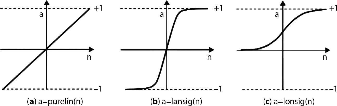
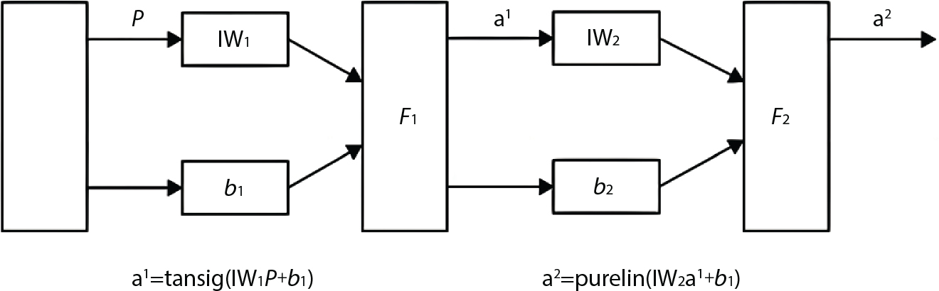
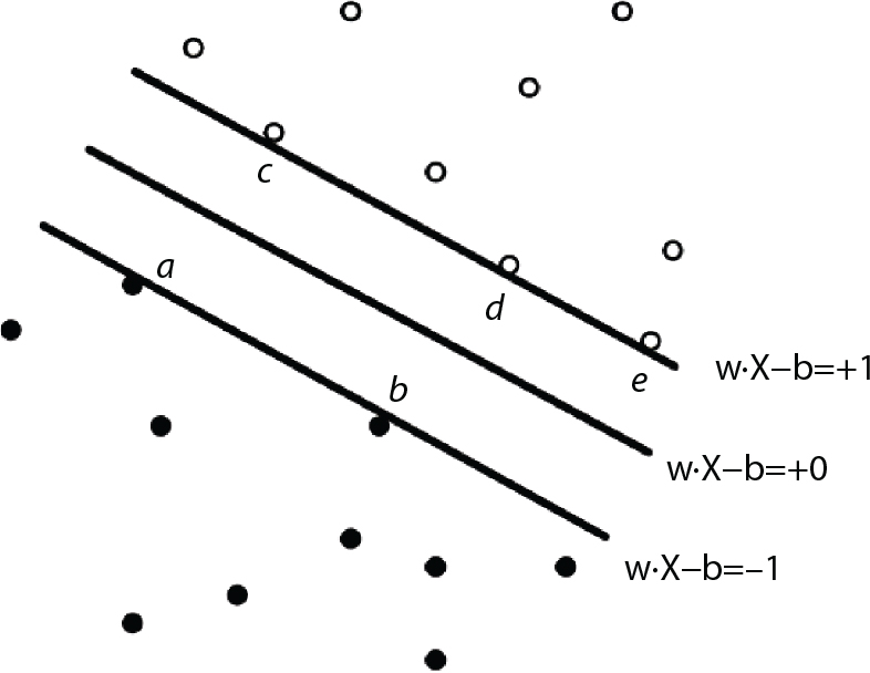
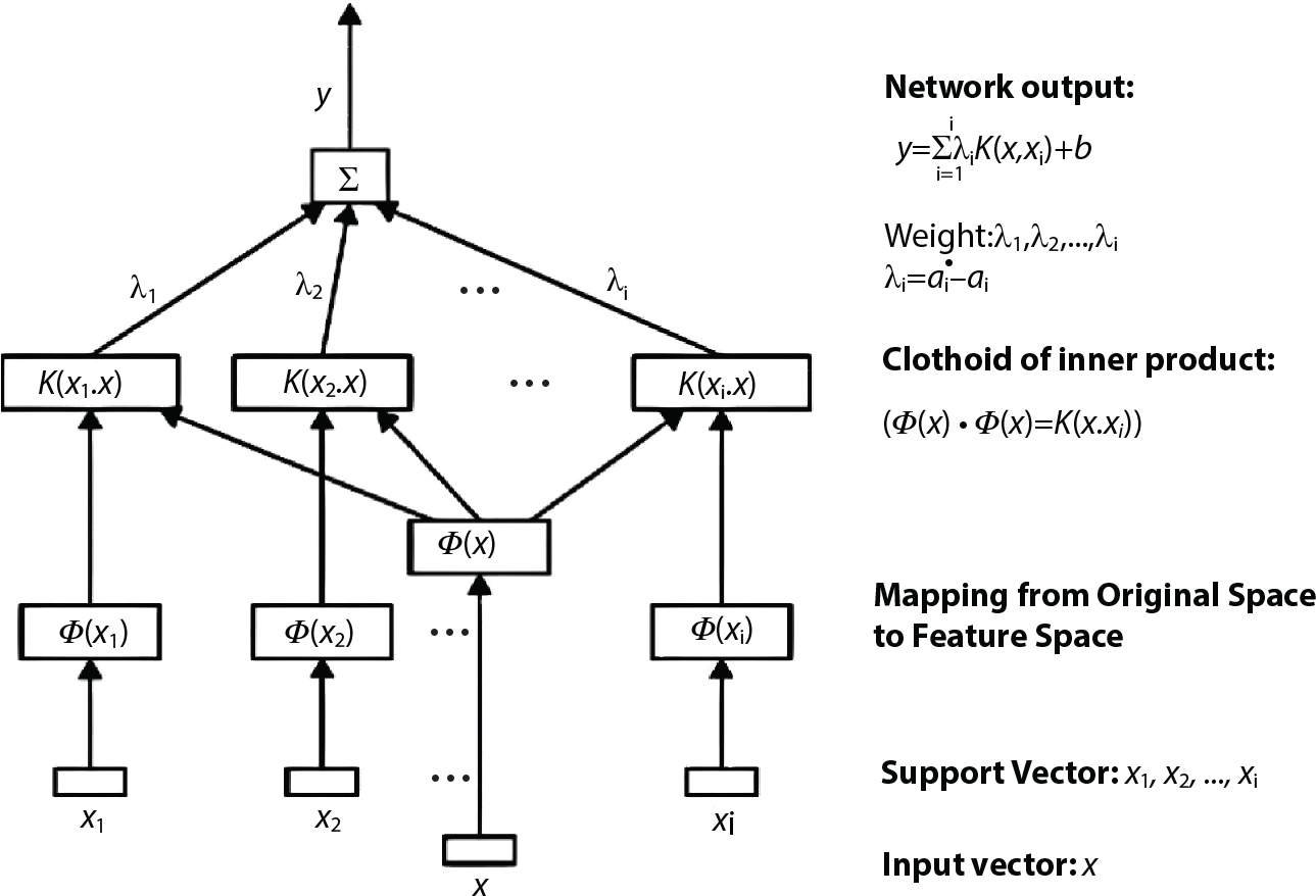
2.6.2 Support Vector Machine
 , and input vector
  . In this way, the first-order partial derivative of the response surface equation constructed by linear kernel, polynomial kernel, RBF kernel and two-layer neural network (Sigmoid) kernel can be deduced. Examples are as follows:
2.7 Example: Risk Evaluation of Construction with Temporary Structure Formwork Support
2.7.1 Basic Information of the Formwork Support Structure
2.7.2 Establishment of Construction Risk Evaluation System
Level A
Level B
Level C
Level D
Level E
Index
Index (S/N)
Key Score (Weight)
Index (S/N)
Key Score (Weight)
Index (S/N)
Key Score (Weight)
Index (S/N)
Key Score (Weight)
Construction risk of formwork support
Safety management (1)
7.38 (0.45)
Safety education (1)
6.28(0.28)
Personnel ability (2)
8.18(0.36)
Safety protection (3)
7.98(0.36)
Onsite construction
9.08 (0.55)
Design scheme (4)
8.15(0.17)
Inspection and acceptance (5)
6.88(0.15)
Dismantling (6)
5.86(0.12)
Dismantling time (1)
6.73(0.58)
Component dismantling (2)
4.96(0.42)
Materials (7)
9.88(0.21)
Steel pipe quality (3)
8.93(0.48)
Fastener quality (4)
9.86(0.52)
Load (8)
7.13(0.15)
Dynamic load (5)
6.21(0.44)
(6)Stacking load (6)
7.97(0.56)
Erection (9)
9.48(0.20)
Support (7)
5.05(0.15)
Bottom horizontal tube (8)
6.14(0.18)
Scissor support (9)
4.16(0.12)
Fastener installation (10)
9.02(0.27)
Position selection (1)
6.07(0.43)
(2)Proper torque (2)
8.06(0.57)
Vertical rods (11)
9.11(0.28)
(3)Aspect (3)
8.14(0.28)
Step distance (4)
8.34(0.29)
Verticality (5)
6.00(0.21)
Connection mode (6)
6.36(0.22)
2.7.4 Index Weighting
Score
Grade
Score
Grade
10
Most important
5
Somewhat important
9
Extremely important
4
Less important
8
Important
3
Some influence
7
Relatively important
2
Small influence
6
Fairly important
1
No influence
μ1
μ2
μ3 (y)
μ4 (h)
Si
Below junior high school
20-29
1-2
<10
0.90
Senior high school and secondary school
30-39
3-4
10-20
0.95
Junior college
40-49
5-10
21-30
0.98
Undergraduate and above
50-60
>10
>30
1.00
2.7.5 Expert Scoring Results and Risk Evaluation Grades
 . After introducing the λ horizontal truncation set, let
  , and the fuzzy interval that can obtain the score value can be expressed as:
Index
x
Index
x
Index
x
Safety education
8.50
Steel pipe quality
6.65
Position selection
7.45
Personnel ability
5.10
Fastener quality
6.15
Proper torque
7.35
Safety protection
7.55
Dynamic load
7.35
Aspect
8.35
Design scheme
9.35
Stacking load
7.00
Step distance
8.55
Inspection and acceptance
7.35
Support
7.20
Verticality
7.80
Dismantling time
8.55
Bottom horizontal tube
5.50
Connection mode
8.00
Component dismantling
8.55
Scissor support
6.65
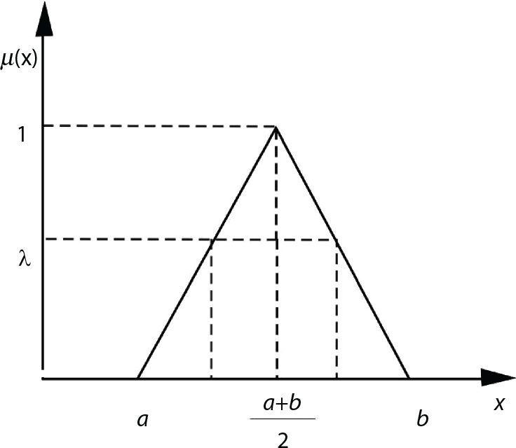
 . If the fuzzy interval of the score value does not belong to [0, 10], then any interval lower than 0 is treated as 0, and any interval higher than 10 as 10.
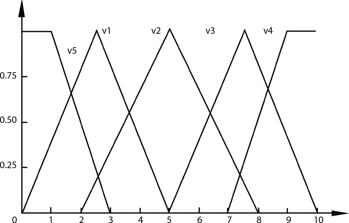
2.7.6 Evaluation of a Fastener-Type Steel Pipe Scaffold
Fastener installation
W10


Position selection
0.43
0.41, 0.49, 0.68, 1.00, 0.79
0.34, 0.34, 0.45, 1.00, 0.48
0.40, 0.53, 0.78, 1.00, 0.62
Proper torque
0.57
0.41, 0.49, 0.69, 1.00, 0.77
0.34, 0.34, 0.46, 0.94, 0.47
0.41, 0.54, 0.80, 0.97, 0.61
Vertical rod
W11


Aspect
0.28
0.41, 0.48, 0.63, 0.94, 0.95
0.39, 0.39, 0.43, 0.78, 0.81
0.34, 0.43, 0.58, 0.90, 0.67
Step distance
0.29
0.40, 0.47, 0.62, 0.91, 0.98
0.39, 0.39, 0.42, 0.73, 0.90
0.33, 0.42, 0.56, 0.86, 0.69
Verticality
0.21
0.43, 0.50, 0.68, 1.00, 0.86
0.39, 0.39, 0.48, 1.00, 0.63
0.36, 0.46, 0.65, 0.94, 0.60
Connection mode
0.22
0.42, 0.49, 0.66, 0.98, 0.89
0.39, 0.39, 0.46, 0.91, 0.69
0.35, 0.45, 0.62, 1.00, 0.62


Material
W7


Steel pipe quality
0.48
0.46, 0.57, 0.84, 1.00, 0.73
0.51, 0.51, 0.81, 1.00, 0.56
0.36, 0.50, 0.83, 0.67, 0.44
Fastener quality
0.52
0.49, 0.61, 0.92, 0.91, 0.68
0.51, 0.51, 0.94, 0.82, 0.51
0.38, 0.55, 1.00, 0.59, 0.40
Erection
W9


Support
0.15
0.42, 0.50, 0.71, 1.00, 0.76
0.40, 0.40, 0.54, 1.00, 0.51
0.44, 0.59, 0.90, 1.00, 0.63
Bottom horizontal tube
0.18
0.49, 0.64, 1.00, 0.77, 0.57
0.43, 0.43, 1.00, 0.56, 0.43
0.48, 0.73, 1.00, 0.58, 0.41
Scissor support
0.12
0.462 0.57, 0.84, 1.00, 0.73
0.51, 0.51, 0.81, 1.00, 0.56
0.43, 0.60, 1.00, 0.81, 0.52
Fastener installation
0.27


Vertical rod
0.28


Construction risk of formwork support
W
B(1)
B(2)
B(3)
Safety management
0.45


Onsite construction
0.55


2.7.7 Discussion and Summary Analysis
References


