The numerical simulation of reliability is an important method for reliability calculation. The Monte-Carlo simulation, also known as random sampling, probability simulation or statistical test, is a method by which stochastic simulation is performed to study objective phenomena [4-1]. Based on the statistical sampling theory, this method is a numerical calculation used to study random variables by means of a computer. Because it is based on probability and mathematical statistical theory, some physicists named it after Monte-Carlo, a city famous for gambling located on the borders of France and Italy, to highlight its randomness. The basic idea of the Monte-Carlo method is that if the probability distribution of state variables is known, then according to the limit state equation of structure, If necessary, the mean μg and standard deviation σg can be calculated according to the N known g(X) values to obtain the reliability index β. For the Monte-Carlo method, a group of random samples is generated based on the probability distribution of basic variables and substituted into the limit state function (LSF) to confirm or rule out structural failure. Finally, the structural failure probability is calculated. This method has the following characteristics: The first four characteristics are not possessed by other reliability calculation methods, while the fifth characteristic becomes less and less prominent as computer technology has continued to improve. Therefore, simulation methods have achieved rapid development in recent years. However, when using the Monte-Carlo method in practice, we must consider: The failure probability of engineering structures can be expressed as Whose structural reliability index is where X = {x1, x2, ⋯, xn}T is a vector with n-dimensional random variables; f(X) = f (x1, x2, ⋯, xn) is the joint probability density function of basic random variable X, and when X represents a group of random variables independent of one another, Thus, Equation (4.2), expressed by means of the Monte-Carlo method, can be written as where N represents the total amount of sampling simulation; when When a 95% confidence interval is selected to limit the sampling error for the Monte-Carlo method, we obtain Or, expressed as relative error ε: Considering that Given ε=0.2, the number of samples taken must satisfy This means that the number N of samples taken is inversely proportional to There are several methods for random number generation, as follows: (1) Linear multiplicative congruence method ① Multiplicative congruence method where a is the multiplier, m is the modulus, and (mod m) means taking remainders after division by m. That is, ② Mixed congruence method where C is the coefficient of correlation between increments xi and xi+1, and its upper bound is When c = 0, (2) Generalized congruence method where If If (3) Random number sequences ① Multiple sequences of random numbers that do not overlap with one another Different initial values are given so that the sequences do not overlap with one another. ② Dual random number sequence For two sequences ③ Reverse order random sequence For two sequences where c represents the cycle length of the random number sequence. When a random sequence is generated by one method, the randomness of this sequence cannot be ensured, making it necessary to check whether it is significantly different from the real uniform random numbers in [0, 1] in terms of properties. If the difference is significant, the samples obtained from the random variables based on the random numbers generated by this random number generator cannot reflect the properties of the random variables, thereby making it impossible to achieve reliable results for random simulation. If a pseudo-random number sequence that has been generated passes a certain randomness test, it could only be said that it is not contradictory to the properties or law of random numbers. We cannot reject it, but it cannot be said that they possess the properties and law of random numbers. Therefore, for the testing of the pseudo-random number sequence, the more tests it passes, the more reliable the random number sequence is. The following are methods for random number testing: (1) Inverse transformation method For the continuous random number x of the distribution function F(x), if there is a uniform random number r in (0, 1), there is also an inverse transform for the generation of x That is, F(x) is a strictly monotonic increasing function, which has an inverse function, so where for the random numbers in (2) Acceptance-rejection sampling method Let the PDF f(x) of random numbers be bounded, with a value range of Steps: Conditions: The Monte-Carlo method is extremely useful. However, if the structural failure probability of an actual engineering structure is less than 10-3, the Monte-Carlo method requires a very large amount of simulation, which occupies a lot of calculation time. That is the main problem with this method in terms of structural reliability analysis. Therefore, during the practical application of the Monte-Carlo method, it is often necessary to use sampling techniques to reduce the variance [4-2] and thus reduce the frequency of simulation. The variance reduction technique is a very important method. It can be divided into dual sampling, conditional expectation sampling, importance sampling, stratified sampling, edge number control and correlated sampling [4-2]. If U represents a set of samples uniformly distributed in [0, 1], and the corresponding basic random variable is X(U), where X obeys the distribution of the probability density function (PDF) f(x1, x2, … xn), there exist I-U and X(I-U) as well, which are negatively correlated with U and X(U). Therefore, the simulation estimation of Equation (4.4) is Apparently, Equation (4.18) is the unbiased estimation of Pf, and the variance of simulation estimation can be expressed as where If there is a conditional expectation E(Pf | xi), then as long as a basic random variable xi. exists, and it is also a random variable, then its sampling simulation estimation can be expressed as follows: Correspondingly, the variance of the simulation estimation is where Y = {xl, x2, …, xi-1, xi+l, …, xn}T; so Therefore, not only does the conditional expectation sampling technique reduce the variance of the sampling simulation, but it is also very beneficial to the calculation of truncated distribution probability in Equation (4.20). If there exists a sampling density function h(X), and the following relation is satisfied then Equation (4.2) can be written in the form of importance sampling Then the unbiased estimation of Equation (4.24) is where When the sampling density function is the simulated variance of Equation (4.26) reaches a minimum. It should be said that Equation (4.27) just provides a way to select h(X), but h(X) is very difficult to select because this depends on the distribution form of the random variables, the LSF and the sampling simulation accuracy [4-3][4-4]. However, Equation (4.26) has both upper and lower bounds, which can be obtained by means of the Cauchy-Schwary inequality, i.e., Equation (4.28) can also be expressed as the ratio of the PDF f(X) of random variables to the sampling probability density function h(X), i.e., This expression provides the boundaries of the sampling function h(X). Obviously, Equation (4.27) is the upper boundary of the sampling function h(X), requiring that h(X) should satisfy the where X⋆ is the maximum likelihood point on the LSF. Considering that the ratio of Equation (4.26) is always greater than or equal to The above observation has been partially reflected in the existing importance sampling methods [4-6][4-7][4-8][4-9][4-10][4-11]. However, there is still the tricky problem of how to effectively determine the importance sampling density function (type and parameters). The concept of stratified sampling [4-12][4-13] is analogous to that of importance sampling because both of them require the samples which contribute a lot to Pf. However, stratified sampling does not change the original density function, but simply divides the sampling interval into further subintervals, keeping different numbers of sampling points in the subintervals so that more samples should be taken from those subintervals which make greater contributions. The domain of integration G(X)<0 is divided into M mutually disjointed subintervals Lj, and from each subinterval, Nj uniform random number vectors r uniformly distributed within this subinterval are taken. Here, Nj represents not only the number of uniform random number vectors generated in the j-th sub-interval, but also the frequency of the uniform random number vectors falling into this subinterval from [0, 1]. In this way, the simulation results for stratified sampling can be written as: The simulated variance is: where In the simulated variance Equation (4.33), it can be proved that if and then Therefore, in order to reduce the simulated variance, the number of samples taken from each subinterval should be directly proportional to the product of the standard deviation and of this subinterval and its volume. Suppose Equation (4.2) can be divided into two parts [4-2]: where Suppose The corresponding simulated variance is: The estimation formula for simulated variance is: As can be seen from Equation (4.38), if y(X) is very close to f(X), i.e., The significance of the control variates method is that if part of the known analytical solution is contained in the problem to be solved, then the variance of sampling simulation can be significantly reduced by removing this part and calculating the difference using the simulation method. Usually, one of the main purposes of simulation is to ascertain the effect of slight changes that take place in the system. Thus, it is necessary to carry out simulation repeatedly. If two tests are independent of each other, then the variance of the difference between the simulation results is the sum of the variances of each simulation; if the same random number is used in the two tests, the test results are highly correlated with each other, thus making it possible to reduce the test variance of the difference between the test results [4-2]. Consider the following two integrals: Their difference is where X1 and X2 are random number vectors with the density function of f1(X) and f2(X), respectively. They are generated by the same set of uniform random number vectors in [0, 1], so Therefore To facilitate the calculation of the estimated value of test variance, the same number of tests, N, is taken for both tests. So then For the LSF of a structure there exists so or where or If there exists an importance sampling density function h(X), as follows Then the failure probability [4-4] in Equations (4.2) and (4.24) can be expressed as or Equations (4.55) and (4.56) are the expression (4.52) of conditional expectation sampling. According to the results of Equation (4.53), Equations (4.55) and (4.56) also have good sampling efficiency. If a normal distribution probability density function is chosen as the sampling density function of xi(i≠ k) in Equation (4.54), then Equations (4.55) and (4.56) will have higher sampling efficiency; during the selection of parameters for the sampling distribution probability density function or For the random variable xi in X ∈ Df, this can be selected according to Equation (4.49) or by the Taylor expansion of Z = G(X); here, xi is allowed to take its value near the boundary domain of Df, and the accumulated deviation will be eliminated in Equation (4.49); therefore, for the selection of xk, it is necessary to consider the univariate form in LSF, as well as the variable with high discreteness in probability distribution. After Equations (4.59) and (4.60) are determined, the importance sampling density function becomes where For the extremal distribution function, If the importance sampling density function is set to a truncated distribution function [4-2], as follows where d represents the truncated value, as shown in Equation (4.49); σ1 is a parameter that varies with the probability distribution of the basic variable x. When the basic variable obeys the normal distribution N(μ, σ2), σ1 can be expressed as Figure 4.1 shows the form of the truncated distribution probability density function; Table 4.1 shows the change of σ1 with σ when G(X)=3.0 – x; as can be seen, the results obtained in Equation (4.63) are obviously better than other results; when the basic variable obeys lognormal distribution, it can be transformed into normal distribution first, before the value of σ1 can be worked out using Equation (4.63). It can then be inverted to lognormal distribution. Therefore, the sampling simulation of where Figure 4.1 Probability density function with truncated distribution. Table 4.1 Simulation results of σ1 versus σ when G(X)=3.0 – x. Note: 1. LSF G(X)= 3.0 – x, x ∼ N (0, o2), Pf = 9.866×1G-10 2. When σ = 0.5, σ1| Equation (4.64) = 0.25, exact value of Pf = 9.866×10⁻¹⁰; When σ = 1.0, σ1| Equation (4.64) = 1.00, exact value of Pf = 1.350×10⁻¹⁰. Table 4.2 Results of different sampling simulation methods. Note: (1) The number in brackets after the variance represents the exponent of 10; 2) LSF Thus, the sampling simulation of Equation (4.61) can be expressed as To sum up, in order to reduce the number of sampling simulations in the Monte-Carlo method and improve sampling efficiency, conditional expectation sampling can be combined with importance sampling to perform a composite sampling simulation to ensure the effectiveness of sampling every time. This also avoids the complexity caused by the use of an optimization method to determine sampling parameters. As a new way, sampling parameters can be determined by the moment method; the effectiveness of sampling simulation can be improved by adopting a normal distribution function for importance sampling and a truncated distribution function for conditional expectation variables; various examples confirm the effectiveness and wide applicability of this improved simulation method. If X space is an original basic random variable space, U space, a standard normally distributed variable space, can be obtained by means of the Rosenblatt transformation [4-14][4-15] x=Txu (u). In U space, the joint PDF f(u) of random variables is monotonous, and u⋆ is the maximum likelihood point on the failure surface, i.e., the minimum distance from the origin of coordinates, which can be obtained by FORM/SORM. This also means that the curvature at u⋆ is always greater than or equal to −1/β [4-16]. P is the reliability index, and β=(u⋆T u⋆)1/2. To make full use of the quadratic effect on the failure surface, the failure function is expanded by Taylor series at u⋆, with the quadratic term taken. So where Gu(u⋆) and Guu (u⋆) are first and second derivatives of G(u) at u⋆. Equation (4.66) is orthogonally transformed, meaning so that zn is parallel to the direction cosines of -Gu(u⋆)/|Gu(u⋆)| at u⋆. H can be obtained by the standard Gram-Schmidt Equation [4-17]. Thus, Equations (4.66) can be expressed as where κ is the eigenvector of matrix This can also be expressed as the relationship with U space, as follows where Tu, x = P · H is the orthogonal transformation matrix for U space and V space. Therefore, V space is only the linear transformation of U space, and is also a standard normally distributed variable space [4-15]. By substituting Equation (4.71) into Equation (4.66), we can establish a failure function for V space: where ann is an element on the nth row and nth column of the matrix A, and An is a vector on the nth row or nth column of the matrix A that does not contain ann. It should be said that Equation (4.72) is a general expression of the failure function with a quadratic effect in V space. For simplification, an approximate parabolic function is usually adopted to replace Equation (4.72). This type of approximate parabolic function is effective in describing the quadratic effect of the surface at u⋆, as follows or Figure 4.2 Approximate parabolic surface of V space. Figure 4.2 shows the approximation of the parabolic surface in V space at u⋆. The importance sampling zone refers to the fact that the samples in this zone have an important contribution to the estimation of Pf, and it is composed of the sampling center and a region with a certain confidence level. In V space, such an importance sampling zone can be represented as an ellipse, as shown in Figure 4.3. According to the symmetry of the approximate parabolic surface and the observation of the importance sampling method, the sampling center is located on the vn axis and within the failure region Df, while the semi-axis length of the ellipse is related to the variance of sampling variables and changes within the geometric properties of the failure surface. Figure 4.3 Important sampling area of V space. (1) Sampling center As shown in Figure 4.3, the position of the sampling ellipse center changes with the principal curvature κi, while the sampling center is located on the vn axis. Its distance from the maximum likelihood point v⋆ on the failure surface is kibi (i.e., Therefore, the parameter ki can be constructed into the following function: where k0 is related to the ratio δ0 of the effective sample region Aeff to the whole sample region Awhole when κi=0. This can be obtained by the following equation: Table 4.3 Relationship between area ratio of sampling ellipse δ0 and k0. Table 4.3 shows the numerical values of k0 corresponding to different δ0 values. (2) Axial length of sampling ellipse As can be seen from Figure 4.3, the semi-axis length of the sampling ellipse on the vn axis can be expressed as where Δβ is a parameter related to the simulation accuracy. Reference [4.20] provides a suitable range of Δβ, i.e., 0.7∼ 1.4. The length of the other half axis of the sampling ellipse can be obtained depending on the geometric properties of the failure surface: where κi,cr can be obtained by equating Equation (4.78b) and (4.78c). Figure 4.4 shows the relationship between the principal curvature κ of the failure surface and the elliptic parameters a, b and k. Figure 4.4 Relationship between principal curvature k and sampling elliptic parameters a, b and k (β=3, Δβ=1.0, δ0=0.8). Choosing an appropriate sampling function is one of the main parts of importance sampling. Because V space is standard normally distributed variable space, an n-dimensional normal distribution probability density function The standard variance of the sampling function involves the confidence level of the samples generated in the importance sampling zone. Let α be the confidence coefficient, and the double-axis length of the sampling ellipse be a confidence interval. The standard variance of sampling will be where αS = 1/Φ-1 [(1+α)/2], and Φ-1[·] is the reversal of the standard normal probability function. Figure 4.5 shows the effect of different confidence coefficients α on the simulation results. As can be seen, an appropriate α value ranges from 0.90 to 0.999, but it should be noted that α also depends on the geometric characteristics of the failure surface. Figure 4.5 Influence of different confidence a on simulation results. Therefore, the importance sampling expression of V space can be expressed as where We can now make a comprehensive comment on the above process of constructing V space by the importance sampling method. As can be seen, the construction of h(v) is related not only to the geometric parameters (maximum likelihood point, gradient and curvature) of the failure surface, but also to parameters of the sampling function (effective sampling zone ratio δ0, effective sampling zone Δβ, confidence coefficient α). The former directly affects the accuracy and efficiency of sampling, but it can be expressed by V-space sampling; the latter plays an important role in the process of constructing h(v), but it seems to be less sensitive to the simulation results given suitable parameters. When parameters are set to δ0 = 0.8, Δβ = 1.0 and α = 0.95 in the following examples, ideal V-space sampling results can be achieved under all failure function conditions. Based on the contents outlined in the previous sections, the simulation process of V-space importance sampling (ISM-V) can be described as follows: A random variable space (U space) can be transformed into another random variable space (V space) through a linear orthogonal transformation matrix so as to reflect the quadratic effect of the failure surface at the maximum likelihood point more accurately. Thus, an importance sampling method (ISM) is established for V space. This type of ISM fully considers the geometric properties of the failure surface (e.g., maximum likelihood point, gradient, curvature, etc.), thus ensuring the validity of samples and improving calculation efficiency. With a wide variety of applications, it is not only used for the convex failure surface, but also for flat or concave failure surfaces; moreover, with increased simulation times, the simulation results show very stable convergence, close to the exact value. For the establishment of a structural LSF by regression SVM, a regression SVM-based ISM can be constructed for structural reliability based on the ISM [4-18][4-19]. By the SVM responding surface equation, a regression SVM-based ISM is developed for the calculation of failure probability: where N represents the number of sampling points; The calculation steps for regression SVM-based ISM are as follows:
4
Numerical Simulation for Reliability
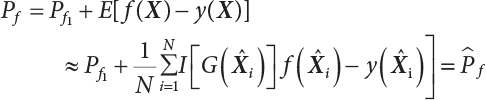
 , a group of random numbers that obeys the probability distribution of state variables, x1, x2, ⋯, xn, is generated by the Monte-Carlo method and substituted into the state function
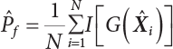
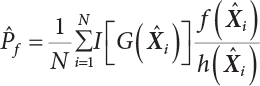
  to work out a random number of the state function. Then, N random numbers of the state function are generated in the same way. If M of the N random numbers are less than or equal to 1, or less than or equal to zero, then when N is large enough, and according to the law of large numbers, the frequency is approximate to the probability. This means that failure probability can be worked out as follows:
4.1 Monte-Carlo Method
 ; G(X) represents a set of LSFs. When G(X)<0, it means that structural failure has occurred; when this is not the case, the structure is safe; Df is a failure zone corresponding to G(X); Φ(·) is a cumulative probability function that obeys standard normal distribution.
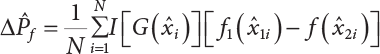
 , or otherwise,
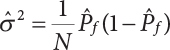
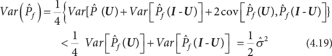
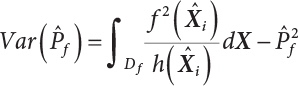
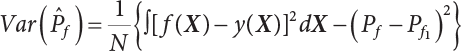
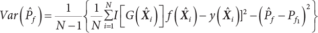
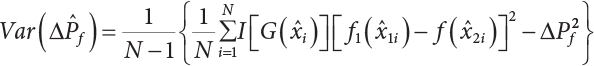
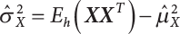
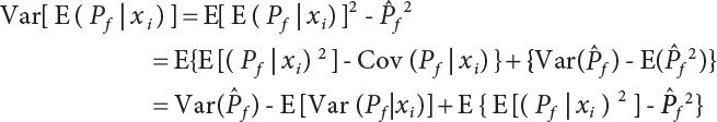
  ; the mark “^” represents the sampling value. So, the sampling variance in Equation (4.4) can be expressed as
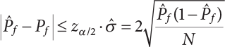
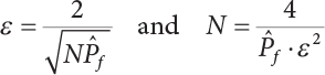
 is usually a small quantity, the above equation can be approximated to:
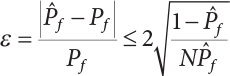
 ; when
  is a small quantity, i.e.,
  , Pf cannot be estimated reliably enough unless N=105; however, the failure probability of engineering structures is usually low, indicating that N must be large enough to make a correct estimation. Obviously, it is very difficult to use the Monte-Carlo method for the reliability analysis of engineering structures in this way. Only by using the variance reduction technique to reduce N can we use the Monte-Carlo method for reliability analysis.
4.1.1 Generation of Random Numbers
 , where m is the remainder. ri is a random number uniformly distributed in [0,1].
 .
.
 , and its upper bound is a minimum.
 is a deterministic function, xi is an integer in
  , and ri is a uniform random number in
  .
.
 , we call it the quadratic congruence method.
 , we call it the additive congruence method.
 ,
, ,
, ,
, they must satisfy
 ,
,  they must satisfy
4.1.2 Test of Random Number Sequences
4.1.3 Generation of Non-Uniform Random Numbers
 .
.
 , so
, so


 , x is accepted as the required random number
4.2 Variance Reduction Techniques
4.2.1 Dual Sampling Technique
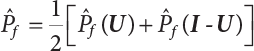
 is negatively correlated with
  ,
,  . Therefore, the variance of the simulation estimation is always smaller than the sampling variance obtained by the Monte-Carlo method. It should be noted that the dual sampling technique does not change the original process of sampling simulation estimation, but merely makes use of the negative correlation among subsamples to reduce the number N of sampling simulations. Therefore, the dual sampling technique can be combined with other variance reduction techniques to further improve the efficiency of the sampling simulation.
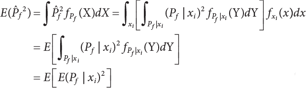
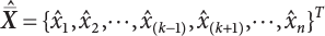
4.2.2 Conditional Expectation Sampling Technique
 in
in  is a variable expected to be estimated. So
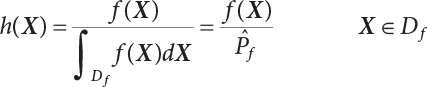
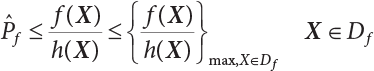
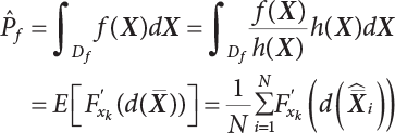
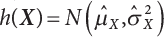
4.2.3 Importance Sampling Technique
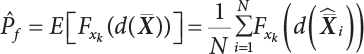
 represents a sample vector taken from the sampling density function h(X); the variance of its sampling simulation is
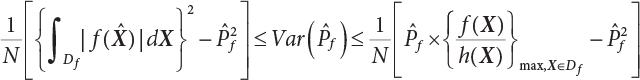
 ratio in the failure zone Df. Moreover, all samples should fall within Df (see Equation (4.23)). At the same time, FU [4-5] has proved the upper boundary of Equation (4.29), as follows
 , and that f(X) can always find such a point in the gradient direction of X⋆ to meet the conditions of Equation (4.27), this point is selected as the subdomain center of the failure zone so that at a given confidence level, the sampling mean obtained from this subdomain meets the conditions of Equation (4.27). This observation is very useful for the construction of sampling function h(X), implying that the sampling center may be in the gradient direction of X⋆ and near X⋆ in the failure zone.
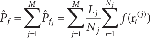
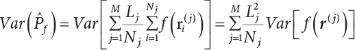
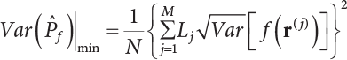
4.2.4 Stratified Sampling Method
 ; correspondingly, the estimated value of simulated variance is:
4.2.5 Control Variates Method

 has an analytical solution. Therefore, only
  can be solved by the simulation method, so
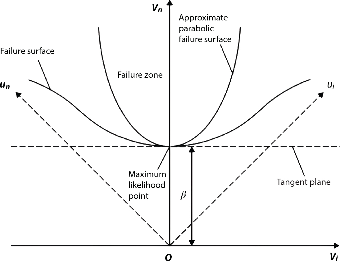
 , then
  . So, y(X) is called the control variate of f(X).
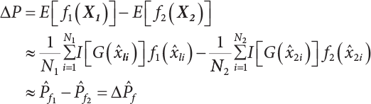
4.2.6 Correlated Sampling Method
 .
.
 and
and  are estimated by means of the expectation estimation method. So
 and
and  are positively correlated with each other. So
4.3 Composite Important Sampling Method
4.3.1 Basic Method
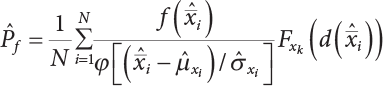
 is the probability value of the random variable xk at
  ; correspondingly, the PDF in Equations (4.52) and (4.53) is
 , the sampling function h(X) is required to satisfy at least the first and second moments of the random variable in the failure zone, i.e.,
 . Therefore, Equation (4.55) can be rewritten as
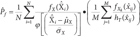
 represents the sample generated by the importance sampling density function; φ[·] is a standard normally distributed probability density function.
4.3.2 Composite Important Sampling
 can be obtained by the deterministic method. For other types of PDF,
  can be obtained by sampling. An effective importance sampling method will be given here.
 and
and  can be expressed as
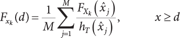
 is a sub-sample generated by hT(x); M represents the number of samples. Table 4.2 shows a comparison of the results achieved by different sampling simulation methods. ISM is the important sampling method, whose sampling function obeys normal distribution; its mean is the “design checking point” and the mean-square error of sampling is set to unit value. IFM is an iteratively faster Monte-Carlo method; IISM is an improved numerical simulation method; AIISM is the IISM with dual sampling technique. As can be seen, IISM reflects the simulated sampling results of Equation (4.64).
N
σ = 0.5
σ = 0.1
σ1 = 0.5 (×10-10)
σ1 = 1.0 (×10-10)
σ1 = 2.0 (×10-10)
Eq. (4.64) (×10-10)
σ1 = 0.5 (×10-3)
σ1 = 1.0 (×10-3)
σ1 = 2.0 (×10-3)
Eq. (4.64) (×10-3)
9.577
7.940
18.480
9.992
1.504
1.316
0.997
1.316
50
10.480
10.127
8.481
9.832
1.187
1.329
1.544
1.329
100
10.420
9.281
7.327
9.826
1.236
1.326
1.339
1.326
200
9.630
9.692
9.297
9.880
1.326
1.343
1.394
1.343
500
9.834
9.898
10.080
9.870
1.234
1.343
1.319
1.343
1000
9.755
9.588
9.430
9.862
1.370
1.348
1.334
1.348
2000
9.902
9.878
10.130
9.866
1.337
1.349
1.340
1.349
5000
9.796
9.751
10.110
9.860
1.340
1.350
1.384
1.350
10000
9.822
9.691
9.994
9.864
1.378
1.350
1.352
1.350
1000000
9.864
9.849
9.901
9.866
1.344
1.350
1.350
1.350
N
ISM
IFM
IISM
AIISM
Pf(×10-3)
Var
Pf(×10-3)
Var
Pf(×10-3)
Var
Pf(×10-3)
Var
10
1.161
2.892 (-7)
0.790
2.520 (-8)
1.316
1.906 (-9)
1.364
1.048 (-11)
50
1.239
1.020 (-7)
1.233
2.005 (-8)
1.329
2.040 (-10)
1.353
2.793 (-11)
100
1.339
7.007 (-8)
1.234
9.233 (-9)
1.326
1.173 (-10)
1.351
2.166 (-11)
200
1.464
3.449 (-8)
1.476
2.989 (-9)
1.343
5.757 (-11)
1.352
1.052 (-11)
50
1.421
1.368 (-8)
1.386
6.252 (-9)
1.343
2.230 (-11)
1.351
4.234 (-12)
1000
1.333
6.311 (-9)
1.375
2.168 (-9)
1.348
1.039 (-11)
1.350
2.125 (-12)
2000
1.323
3.030 (-9)
1.363
9.838 (-10)
1.349
5.488 (-12)
1.350
1.025 (-12)
5000
1.368
1.235 (-9)
1.336
2.952 (-10)
1.350
2.164 (-12)
1.350
3.895 (-13)
10000
1.360
6.119 (-10)
1.342
1.332 (-10)
1.350
1.087 (-12)
1.350
1.888 (-13)
1000000
1.350
6.169 (-12)
1.346
2.218 (-12)
1.350
1.070 (-14)
1.350
1.915 (-15)
 when n=1.
4.3.3 Calculation Steps
 for the importance sampling density function according to Equations (4.57) and (4.58);
 from
from  , and calculate the truncated value di through Equation (4.49);
 from Equation (4.62), and calculate
  ;
;
 using Equation (4.64);
 and
and  ;
;
4.4 Importance Sampling Method in V Space
4.4.1 V Space
 ,
,  . The principal curvature of the failure function at u⋆ can then be taken into consideration. According to the characteristic equation, we get
 , i.e., the diagonal matrix of principal curvature.
  is the orthogonal eigenvector matrix of
  , while
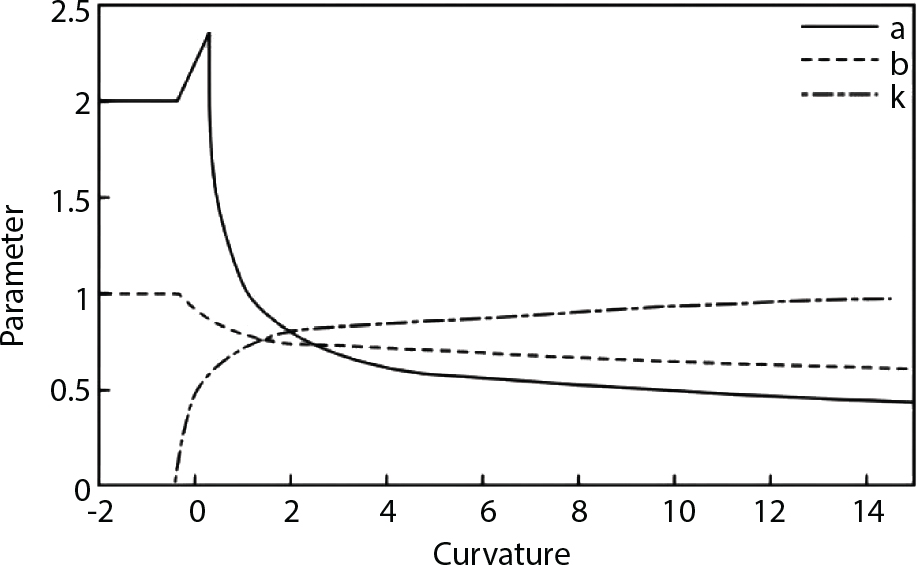
  is a (n-1)×(n-1)-order matrix obtained from the matrix A with the nth row and nth column deleted; therefore, the new coordinate system for these variables corresponds to the main curvature coordinates. So
4.4.2 Importance Sampling Area
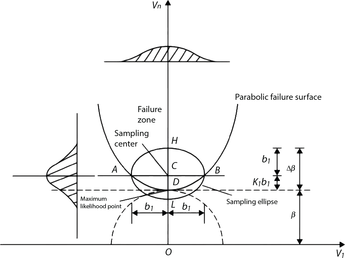
 in Figure 4.3), where bi represents the semi-axis length of the sampling ellipse on the vn axis, and parameter ki should satisfy the following conditions:
δ0
0.50
0.55
0.60
0.65
0.70
0.75
0.80
0.85
0.90
0.95
0.99
1.00
k0
0.000
0.079
0.158
0.238
0.320
0.404
0.492
0.585
0.687
0.805
0.934
1.000
4.4.3 Importance Sampling Function
 can be selected as the importance sampling function h(v). The mean of the sampling function is
 is the sample vector generated by the sampling function h(v).
4.4.4 Simulation Procedure
 from h (v) (Equation (4.81);
 into
into  and
and  by Tuv and Rosenblatt transformation;
 ratio;
 using Equation (4.81).
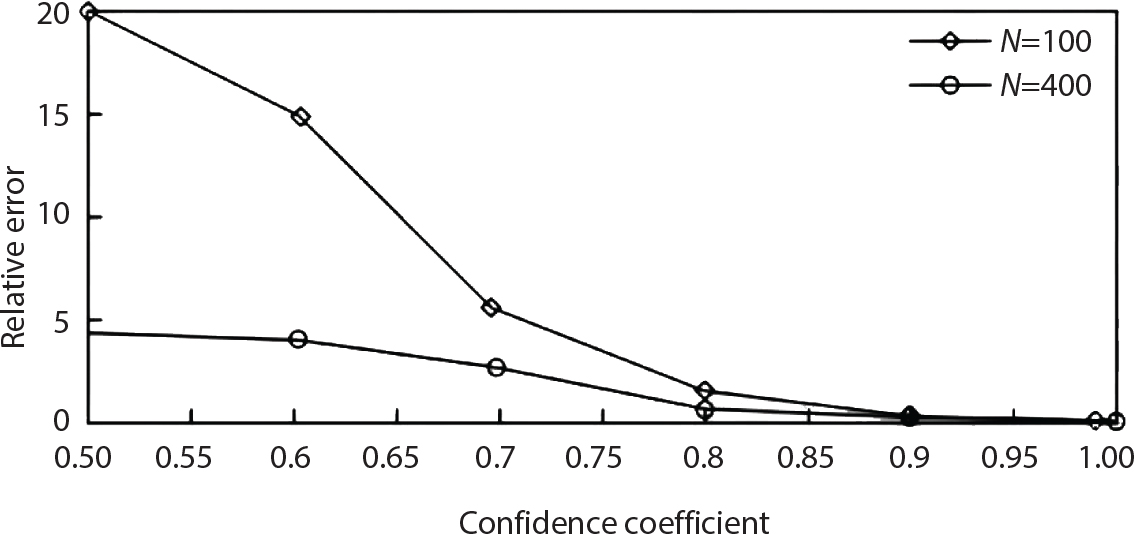
4.4.5 Evaluation
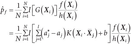
4.5 SVM Importance Sampling Method
 represents support vectors; l represents the number of support vectors; N represents the sampling frequency; f(X) is the joint density function of variables; h(X) is the importance sampling density function; Xi is represents the samples generated by the importance sampling function. K() is the Kelvin function.
 with average point taken normally;
 ;
;
References