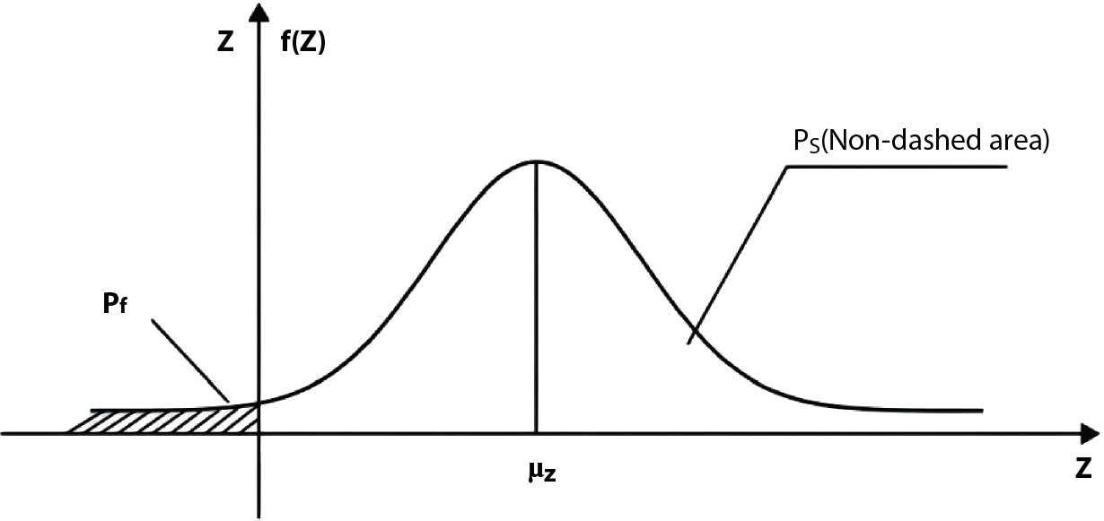
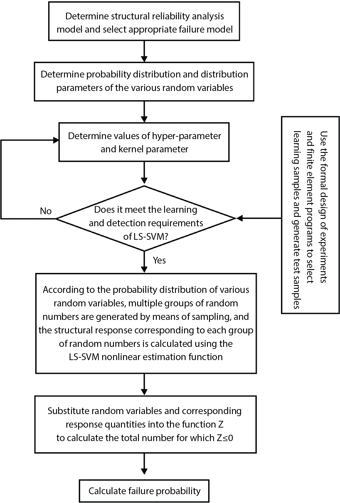
The reliability of engineering structures can be characterized by reliability probability or failure probability. Structural reliability can be measured by means of the theory of reliability. Structural reliability is defined as the probability of fulfilling a certain preset function within the prescribed time under the specified conditions. In contrast, if the structure fails to fulfill a certain preset function, then the corresponding probability can be called structural failure probability. Generally, the reliability and failure are two events which are incompatible with each other. Therefore, structural reliability probability and failure probability are complementary [3-1]. For the convenience of calculation and expression, structural failure probability is often used to measure structural reliability during structural reliability analysis. The core of structural reliability analysis lies in calculating structural failure probability according to the statistical characteristics of random variables and the limit state equation of the structure. In structural reliability analysis, the working state of the structure is generally described by a function. When there are n random variables The safety probability that the structure fulfills the present function under the specified conditions is represented by Ps; at the same time, if the structure fails to fulfill the preset function, then the corresponding probability is called structural failure probability, represented by Pf. Structural reliability and failure are two events incompatible with each other, and there is a complementary relationship between them, i.e., Ps + Pf = 1. Because structural failure is an event of small probability (Pf is usually less than 0.001), structural failure probability is often used to measure structural reliability, for the convenience of calculation and expression. Let the joint probability density function corresponding to the basic random variable In practical calculations, when there are multiple basic random variables in the function, the limit state function is nonlinear, and variables are not independent of one another, making the above equation difficult to solve directly. Therefore, this direct integration method is not usually adopted. Instead, a simple approximation method is applied, and for all random variables, only their digital eigenvalues are considered, with their statistical characteristics described through mean and variance. Therefore, the reliability index β is introduced and calculated in order to compute the corresponding failure probability. First, suppose the function variable Z obeys a normal distribution; its mean is μz and its mean-square error is σz. Therefore, its probability density function is as follows The structural failure probability is represented by the dashed area in Figure 3.1. The expression of the failure probability is as follows Figure 3.1 Diagram of structure failure probability. Notation β is introduced. Let Equation (3.4) can be converted into The relationship between β and reliability can be expressed by the following equation The dimensionless coefficient β in the equation is the above-mentioned reliability index. For structural reliability, it can be expressed as where Z = G(X) is the limit state function, Z < 0 (failure), while Z > 0 (safety), and Z = 0 is the critical state. Df represents the failure zone corresponding to Z < 0, and f(X) represents the joint probability density function (PDF) of random variables. Φ(•) is the cumulation probability function (CDF) of standard Gauss distribution. The structural reliability theory should therefore be used to solve the following four problems: A probabilistic design method fully considering the above four problems is called level IV, while a method considering the first three methods only is called level III. This is an ideal aspect of structural design; after simplification in different ways, it can be called level II, level I, etc. The current structural design code remains at level II. The first-order second-moment method is a method by which the linear term in Taylor’s expansion and the first two moments of random variables (first moment μ and second moment σ) are adopted for calculation. Common first-order second-moment methods include the central point method [3-2] and the checking point method. For the limit state function of a structure (1) When Z is a linear function where ai(i = 0, 1, 2, ……, n) is a constant. So, (2) When Z is a nonlinear function Z is expanded into Taylor’s series at the central point, with the linear term taken. (3) When Z is non-normally distributed Let Case 1: If Z = R − S, let the transformation Currently, the R, S plane represents the distance from the central point to Z′ = 0, respectively. Apparently, there is an error between the distance from the central point to the Z′ = 0 plane and the distance to Z′ = 0. This error increases with the increasing nonlinearity. Case 2: If both R, S obey lognormal distribution, respectively, and the limit state function is expressed as Z = ln R − ln S, then, Z obeys normal distribution, and its mean and variance are When both δR, δS are less than 0.3, respectively, or nearly equal, (4) Evaluation Table 3.1 Relationship between reliability index and failure probability Pf. The linearization point of the checking point method is located at the failure boundary to overcome the problems with the central point method. It is also the location of the design checking point X* (where the distance from the origin of the coordinates to the limit state surface is the shortest) corresponding to the maximum possible failure probability of the structure. This kind of first-order second-moment method is known as the checking point method [3-3] or improved first-order second-moment method, and is the basis for structural reliability index calculations. The checking point method could be used in X-space or U-space. (1) X-space A linearized limit state equation can be established by selecting the design checking point Because X* is situated on the failure boundary, there is So Because The sensitivity coefficient, So This can also be expressed as It has There is a total of n equations in the above equation, where (2) U-space Let The proposition of βmin may be calculated, or it can be expressed in optimal form in U space. Condition Where f(U) represents the probability density function of U. Thus, Equation (3.24) can be expressed as Therefore, we can construct a function, Z(u) = f(u) + λg(u), where λ is a Lagrange coefficient where So When g(u) = g(u0) + gu(u0)(u−u0), we have So, the iteration for the design checking point is where Because u* is a design checking point on Z=0, so We have The above solution process is: Comparison with the central point method, there are The Breitung method [3-4] [3-5] could treat with random variables by mapping transformation and analyze the problem in standard space. Let Y be an independent standard normal random variable, expand the function Z into Taylor’s series at the checking point, and take the first and second terms to obtain: Let the unit vector be Because So αX is used to construct an orthogonal matrix H, HT · H = I, αX is a certain column of H, set to n for orthogonal transformation of Y space to U space. Equation (3.34) is substituted into (3.32). It is noted that where (HTQH)n−1 is an n-1-order matrix generated from HTQH with the nth row and nth column ruled out, The joint probability density function of Y is By substituting Equation (3.34) into (3.36), we get Structural failure probability For Equation (3.35), according to Equations (3.37) and (3.38), the failure probability of the second-order second-moment method is Let The above equation can also be written as By substituting Equation (3.41) into (3.39), we get The integrand in Equation (3.42) is compared with the normal joint probability density function with a mean value of 0 and a covariance matrix of If the reliability index of the first-order second-moment method is obtained, then the failure probability of the second-order second-moment method can be obtained from Equation (3.43). Where κi is the eigenvalue of the real symmetric matrix The following steps can be applied in the above derivation process: The Laplace method is a type of second-order second-moment method, in which the second-order partial derivative of nonlinear functions is adopted. When Y obeys independent standard normal distribution, the structural failure probability is When the Laplace asymptotic integral method is used to calculate the above multiple integrals, the Laplace integral containing large parameters is adopted: The properties of integral Equation (3.46) are fully determined by the properties in the neighborhood of the integrand maximum. If functions h(x) and g(x) are twice continuously differentiable, while p(x) is continuous and h(x) only reaches its maximum at x*, a point on the boundary of the integral domain, Equation (3.46) can be approximately expressed as where Matrix A large number, λ(λ → +∞), is chosen for transformation The Jacobi determinant of the transformation is det JYV = λn. By substituting Equation (3.50) into Equation (3.47), we get Equation (3.51) is also a Laplace integral shown in (3.46), and If the function is twice differentiable, then the asymptotic integral value of Equation (3.51) is where Matrix B1(v*) is an adjoint matrix of matrix C1(v*) By substituting Equation (3.54) into (3.53), we get where Considering that β is generally a relatively large positive value, φ(β) ≈ βΦ(−β), Equation (3.54) can be written as The following steps can be applied in the above derivation process: In 1948, Shannon introduced the concept of thermodynamics into the information theory. If a random variable has n possible results, the probability of each result is pi. To measure the uncertainty of this event, the following function is introduced: where c is a constant greater than 0, meaning H is also greater than 0. H is called the Shannon entropy. A certain event has only one result, pi=1, and there is no uncertainty, so H = 0. If random events obey continuous distribution with the probability density function of f(x), then the Shannon entropy is The Shannon entropy is used to measure the uncertainty of an event before it occurs; after the occurrence of the event, the Shannon entropy is used to measure the information obtained from it. This is used to measure the uncertainty of an event or the amount of information it contains. Under given conditions, there exists a distribution among all possible probability distributions that enables information entropy to reach a maximum. This is called Jaynes maximum entropy principle. The information entropy is maximized under known additional information constraints, and the obtained probability distribution is minimally biased, thus finding a way to construct an “optimal” probability distribution. We consider taking the first m–order origin moment of a random variable x as constraints, i.e., the information entropy is maximized by meeting the conditions in the equation below Using the Lagrange multiplier method, as well as Equations (3.60) and (3.61), a modified function is introduced At the stable point there is Equation (3.62) is equivalent to the central moment of a given x Usually, we can get the first four-order central moments of X, as follows where Csx is the skewness coefficient and Ckx is the kurtosis coefficient. In Pearson’s system, it is considered that the probability density function fX(x) of a random variable x is determined by the ordinary differential equation below: By integrating Equation (3.66), we can obtain a family of curves. Equation (3.66) is a general form of Pearson’s family of curves, in which the parameters can be expressed by the first four-order central moment of X, as follows The following recursive relation exists between all-order central moments of the family of curves: Each order may be totally different from one another in terms of μxi, so x is converted into a standard random variable, According to Equation (3.69) and (3.70), it is noted that μy = 0, σy = 1, vyi = μyi. The first four moments of y are as follows For the standard random variable y, and with determined Pearson system parameters, Equation (3.67) can be written as Equation (3.71) can be used to derive higher-order moments if x in Equation (3.71) is replaced by y. Let the structural function be Z = g(X), where the statistical parameters of Xi in By expanding Z into Taylor’s series at the checking point and taking the quadratic term, we can get According to Equation (3.72), the first four moments of ZQ can be calculated as follows: Z is standardized as The coefficient in f(y) can be calculated. The structural failure probability is The following calculation steps can be applied in the above derivation process: If the moments of two random variables correspond to each other, then they also have the same probability distribution and eigenvalue. With the moments as constraints in a given inner product space, the undetermined coefficients of probability density function polynomials can be calculated, thus making it possible to determine the probability distribution form of Z and calculate the structural failure probability. Let the function f(x) be continuous in [a, b], and pi(x)(i = 0, 1, ⋯, m) be m+1 linearly independent continuous function in [a, b]. Its linear combination According to Or rewritten as where the elements of matrix A and the components of vector b are as follows Matrix A is an m+1-order nonsingular matrix, meaning Equation (3.78) has a unique solution. Let the probability density function of random variable x be f(x). If pi(x) = xi, ρ(x) = 1, then the following can be derived from Equations (3.78), (3.79) and (3.80) If the every-order origin moment of x is known, λi(i = 0, 1, ⋯, m) can be worked out by solving Equation (3.77), with the polynomial of least square approximation, p(x), obtained, leading to The following steps can be applied in the above derivation process: The random variables in the reliability calculation of engineering structures do not always obey a normal distribution, whereas the definition of reliability index is based on the premise that random variables obey a normal distribution. Therefore, when the random variables do not obey normal distribution, it is usually necessary to transform these variables to solve the reliability index. The following methods are usually used to convert random variables into normal random variables. The R-F (Rackwitz & Fiessler) method [3-6] is designed to solve the problem of arbitrary distribution of random variables. The following conditions are proposed in this method: (1) At the design checking point, F(x*)=Fnormal(x*), and the probability distribution functions before and after transformation are equal; (2) at the design checking point, f(x*)=fnormal(x*), and the probability density functions before and after transformation are equal; under this condition, β and Pf can be calculated by the checking point method for normal variables. So, from condition (1), the following can be obtained From condition (2), the following can be obtained So The following steps can be applied in the above derivation process: The Rosenblatt transformation [3-7] is designed to solve the problem of random variables with arbitrary distribution and correlation. According to the principle of conditional probability, the non-normal random variables are transformed into independent standard normal random variables. Conditions: According to condition (1), if ri is an independent standard normal variable, then R = TX, where T refers to the Rosenblatt transformation where Conditional probability density function where Therefore, the following can be derived by the inverting method The above inverting method usually needs to be applied in combination with the numerical method, making it rather difficult to use; here, For example, n = 2 Apparently, this free combination leads to a difference in the method of solving for X. But fortunately, the conditional probability density function or distribution function is not always known in engineering practice. Often, some estimates or correlations can be utilized. Particularly, when xi is independent, The Rosenblatt transformation can transform one type of variable distribution into another type, so In particular, when u is an independent standard normal variable, there is Transformed by Invert into In U-space, where: Jij is a coefficient of Jacobian matrix, and the Inverse matrix is as follows: So, for the linear limit state equations, the relationship between them is After the above transformation, the checking point method can be used to calculate β and Pf. This is usually an iterative solution process. The following steps can be applied in the above derivation process: The P-H (Paloheimo-Hannus) method [3-8] lies between the central point method and the checking point method. Its basic starting point is as follows: (1) arbitrarily distributed random variables; (2) the limit state function (LSF) of multiple random variables. For LSF is g(X), if there is where For For β is the safety index, which can be worked out according to LSF g(X) = 0. Under multivariable conditions, it is considered that And where βi can be obtained by The following steps can be applied in the above derivation process: For the modified P-H method [3-9], which is based on the P-H method, In a complex structure, when the relationship between a function g(X) and a random variable X cannot be expressed explicitly, an appropriate and explicit functional expression can be used to approximately express g(X). That is, the smallest number of deterministic finite numerical values are used to fit a response surface to replace the unknown real limit state surface so as to calculate its reliability by any known method (as shown in Figure 3.2). This is known as the responding surface method, proposed and applied by Box and Wilson [3-10]. The responding surface method is a comprehensive statistical test technique, in which an inference method is used to reconstruct the limit state equation near the checking point. For the reconstruction of a structurally complex approximate function, this means that a series of variable values are designed, with every group of variable values forming a test point. The structure is then calculated point by point to obtain a series of corresponding function values. These variable and function values can be used to reconstruct a clearly expressed functional relationship to calculate the structural reliability or failure probability [3-11][3-12]. Figure 3.2 Responding surface function. For n random variables x1, x2, …, xn, a lot of research findings show that due consideration needs to be given to any of the following: simplicity, flexibility, calculation efficiency and accuracy. A quadratic polynomial exclusive of cross terms is usually adopted as the analytical expression of a responding surface, as follows where a, bi and ci are all undetermined coefficients, with a total number of 2n+1. For each group of random design variables x1, x2, …, xn corresponds to a response For the responding surface method, the key is to fit the limit state function to the structure. A clear functional relationship can be established by fitting according to variable values and function values to calculate the structural reliability or failure probability. The traditional responding surface method can be used to reconstruct the approximate limit state to work out the checking point X* and reliability index β. The steps are as follows Given an initial value point The function values are worked out by finite element simulation, as follows: If the conditions fail to be met, a new initial value point needs to be selected using the interpolation method During the reconstruction of LSF by the responding surface method, a rough approximate quadratic function is reconstructed based on the initial test results. Then, under the condition that the convergence conditions are met, the function is expanded, obtaining a new initial value point. According to the new test results, the reconstructed function is constantly adjusted so that the initial value point gradually approaches the checking point. The expression that meets the convergence conditions represents the real surface behavior near the checking point. At present, there are more responding surface reconstruction methods than polynomial methods. AI methods, such as the neural network method and the SVM method, can also be used for responding surface construction. 1) Principle of function estimation On the basis of a set of fixed training sample sets {(xj, yj}; j=1, 2, …, l}, xj∈Rn and yj∈R, the samples from the original space Rn are mapped to the feature space Rnh using a nonlinear mapping Ψ(·), Ψ(x) = {φ(x1), φ(x2), ⋯, φ(xl)}. Optimal decision functions y(x) = wTφ(x) + b, w ∈ Rnh and b ∈ R are constructed in this high dimensional feature space. Then, the principle of Structural Risk Minimization (SRM) is used to find the weight vector w and deviation b, i.e., by minimizing the objective function where, the error vectors ej ∈ R and γ are adjustable hyper-parameters. Defining the Lagrange function to solve the optimization issue above Where, the Lagrangian multiplier αj ∈ R; according to Karush-Kuhn-Tucker (KKT) conditions: The following equation can be established: The symmetric functions[3-13] defining the Mercer conditions for kernel functions: According to Equation (3.103), the optimization issue is transformed into linear equations: Where, Different support vector machines can be constructed by using different kernel functions. Common kernel forms include: Compared with the standard SVM, the least squares support vector machine (LS-SVM) replaces inequality constraints with equality constraints. With its fast solution speed, this algorithm can be transformed for solving linear equations. 2) Response Surface Methodology Combined with LS-SVM A response surface analysis method for structural reliability based on LS-SVM is hereby proposed to solve the problem of weak function approximation of the response surface method. As a coupled form of the LS-SVM, FEA and Monte-Carlo numerical simulation methods, this method creates a new concept for structural reliability analysis. The LS-SVM program and Monte-Carlo simulation are compiled using MATLAB; the response (such as stress or displacement) of the structure is calculated using the finite element method, with all three integrated into a structural reliability analysis system. See Figure 3.3 for the program block diagram. First, the structure is analyzed to determine the main failure modes; then the input vectors of the learning samples are obtained by an orthogonal experimental design method based on the probability distribution parameters of basic random variables. The structural response values of the input vectors of the learning samples are then obtained using standard finite element programs, such as ANSYS, SAP, or similar, to finally determine the learning samples. Next, the hyper-parameters and kernel parameters are determined using the cross validation method, so that the estimated LS-SVM value for the learning samples approaches the calculation results using the finite element method. The test samples are generated by means of sampling; a check is then required of whether the detection requirements of LS-SVM have been met or not. If not, the values of the hyper-parameters and kernel function parameters need to be adjusted until the requirements above are met, thus establishing a nonlinear mapping relationship between structural action and response. Finally, the failure probability of the structure is determined by the Monte-Carlo method and the LS-SVM nonlinear estimation function. Figure 3.3 Response surface method based on LS-SVM. 3) Generation and initialization of learning samples To establish the nonlinear mapping relationship between structural action (input) and response (output) using LS-SVM, the learning samples of the LS-SVM must be selected or designed based on the specific purpose. If the complete combination method is used, there will be an excessive number of training samples, which will in turn lead to excessive workload. In this test, learning samples were selected using an orthogonal experimental design. Each random variable in the design sample is evenly selected at n levels within the range [mi − 3σi, mi + 3σi], with the value of n depending on the number of random variables. To be more specific, mi and σi are the mean and standard deviations of each random variable. For a normally distributed random variable, the probability that its value deviates from the mean by more than 3 standard deviations is not greater than 0.13%. According to this statistical theory, the above learning samples are highly representative. To eliminate the influence of various factors caused by differences in dimensions and units, the input and output of the sample are normalized by the following equation: Where, zi and yi are the variables before and after normalization, and zmin and zmax are the minimum and maximum values of z. 1) Example 1: Linear limit state equation The linear limit state function is According to Figure 3.4, as the number of variables n increases, the effect of reducing the number of valid element calculations using the improved method becomes more pronounced, indicating that the actual effect of the improved method is related to the number of variables. Figure 3.4 Number of FEM calculations. 2) Example 2: Nonlinear limit state equation If we choose the following three nonlinear limit state equations and calculate the corresponding reliability using different kernel functions. The results are shown in Table 3.2. Example 2-1: Example 2-2: g(X) = 1 + x1x2 − x2, where x1 ∼ LN(2, 0.42) and x2 ∼ N(4, 0.82). Example 2-3: 3) Example 3 [3-14] : Portal plane frame In the portal plane frame shown in Figure 3.5, the elastic modulus of each unit is E = 2.0×10⁶ kN/m2, and the relationship between inertial moment and cross-sectional area is Table 3.2 Comparison of results. Figure 3.5 Portal frame calculation diagram. Table 3.3 Probabilistic characteristics of the random variables in Example 3. The limit state equation can be expressed as Where, [u]=1cm is the maximum allowable horizontal displacement, and the relationship between u3 and each random variable cannot be clearly expressed. Firstly, learning samples need to be designed, and random variables selected from 5 levels {mi −3σi, mi −1.5σi, mi, mi + 1.5σi, mi + 3σi} to create a 3-factor, 5-level orthogonal experimental design. 25 groups of random variables are selected, which are also taken as the input of the finite element program for calculating the horizontal displacements of Node 3, so as to obtain a learning sample for the LS-SVM. The 25 learning samples are normalized according to Equation (3.105), and then input into the prediction model. LS-SVM is used for sample learning. In consideration of the favorable statistical performance of the radial basis function [3-15], this is selected for LS-SVM learning as Where, the εRMS of the learning sample is 2.027×10⁻⁵ and the εRMS of the test sample is 3.9×10⁻³. See Table 3.4 for the comparison between the FEM calculation results of OFEM and the estimated LS-SVM function values After learning and detecting, A1, A2 and P will generate random sampling points according to their probability distributions and the Monte-Carlo principle. Here, N= 100,000 sampling points are taken, and A1, A2 and P form the input vectors of the LS-SVM. By inputting these vectors into the learned estimation function relational expression, 100,000 displacement values of Node 3 can be obtained. If this is substituted into the function Z shown in Equation (3.107), then the number of samples nf for Z < 0 can be obtained, and the failure probability is Table 3.4 LS-SVM learning results. 4) Example 4 [3-14]: Plane frame structure In the calculation diagram of a plane frame structure for a 3-span 12-storey building (as shown in Figure 3.6), the elastic modulus of each unit is E = 2.0×10⁷kN/m2, and the relationship between the unit section inertial moment and the section area is Figure 3.6 Calculation diagram for Example 4. Table 3.5 Probabilistic characteristics of random variables in Example 4. Table 3.6 Effect of sample numbers on calculated results. Assuming normal conditions and a maximum allowable deformation [u]=9.6cm, the following limit state equation can be established according to the code: No explicit relationship is established between uA and the random variables. To study the influence of the number of learning samples l on the calculation results for failure probability, 5 and 7 levels of each random variable were taken, i.e. {mi − 3σi, mi − 1.5σi, mi, mi + 1.5σi, mi + 3σi} and {mi-3σi, mi-2σi, mi–σi, mi, mi + σi, mi + 2σi, mi + 3σi}; an orthogonal experimental design with 6 factors and 5 levels, and one with 6 factors and 7 levels were carried out. 25 and 49 learning samples were selected, respectively, and the failure probability of the structure was calculated using the response surface method based on LS-SVM. See Table 3.6 for the results. To be specific, Pf was obtained following N=100 000 iterations, and the average error εRMS was calculated using Equation (3.108). As learnt from Table 3.6, a correct mapping relationship is established by LS-SVM between 6 random variables and the structural response uA. The response surface method based on LS-SVM is insensitive to changes in sample number. It can thus be seen that this method has strong learning ability for small samples and can greatly reduce the workload of FEA. The failure probability Pf = 7.309×10⁻² obtained by the traditional response surface method is used in Literature [3-14], while the failure probability obtained after 2,000 iterations is simulated using the importance sampling method.
3
Reliability Analysis Method
 affecting structural reliability, the working state of the structure is expressed by Equation (3.1).
 in the structure be
  . The structural function is shown as Equation (3.1). According to the definition of structural reliability and the basic principle of probability theory, structural failure probability can be expressed as
3.1 First-Order Second-Moment Method
3.1.1 Central Point Method

 . As n increases, the distribution of Z becomes asymptotically normal. Therefore
 transform X space into U space. According to the central limit theorem, U is normal space and the above conclusion can still be drawn. There are the following cases.
 ,
,  , so
, so  . Then, the safety index is
β
1.0
1.5
2.0
2.5
3.0
3.5
4.0
5.0
Pf
1.587×10⁻¹
6.681×10⁻²
2.275×10⁻²
6.21×10⁻³
1.35×10⁻⁴
2.326×10⁻⁴
3.167×10⁻⁵
2.867×10⁻⁷
3.1.2 Checking Point Method
 .
.


 , there are

 , represents the relative influence of the ith variable on the entire standard deviation. And
  .
.

 and β are unknown numbers, totaling n + 1. This needs to be solved by an iterative method. The specific steps are as follows:


 from
from 

 into Z(X), and calculate
 , and
, and  , go to 9); otherwise, calculate the Δ-value
  , and estimate a new β value according to
  , and then repeat 3) ∼ 7) until
  .
.
 , so E(ui) = 0. We have the limit state function from Equation (3.20)


 , so f(u) → max.


 represents direction cosines of design checking point u*. fu(u) and gu(u) is the derivative of f(u) and g(u), respectively.
  .
.


 , and X* = μX + αβσX
3.1.3 Evaluation
3.2 Second-Order Second-Moment Method
3.2.1 Breitung Method
 , and
, and  , Equation (3.30) can be written as
 , αX = (0, 0, ⋯, 0, 1)T, so Equation (3.32) can be rewritten as
 .
.
 , and expand InΦ(t – β) by Taylor’s series at t = 0 and take the first term to obtain
 . Equation (3.42) can be simplified as
 , and approximately describes the principal curvature of the limit state surface in the ith direction.
 in Equation (3.31)
3.2.2 Laplace Asymptotic Method
 is an adjoint matrix of matrix
 ,
,  .
.
 is an adjoint matrix of
 in Equation (3.30)
 in Equation (3.57)
 det C
det C
3.2.3 Maximum Entropy Method
 , i.e.,
  . Let
. Let  ,
,  and the maximum entropy probability density function can be obtained as follows,
 , to avoid interrupting the solving process during calculation. There is a relationship between x and y in terms of their every-order central moment
 are
are  , while the first four-order central moments are
  .
.
 . The maximum entropy probability density function of random variable Y meeting the constraint condition remains in the form of Equation (3.63). By substituting Equations (3.73) and (3.74) into Equation (3.61), we get a system of integral equations
3.2.4 Optimal Quadratic Approximation Method
 is utilized to approximate f(x) so that the, integral
  where λi(i = 0, 1, ⋯, m) is the coefficient and ρ(x) is the weight function in [a, b]. This is the least square approximation problem.
 , the essential condition for the extreme value of the multivariate function, linear equations with determined coefficients can be obtained as follows
 in Equation (3.70)
3.3 Reliability Analysis of Random Variables Disobeying Normal Distribution
3.3.1 R-F Method


3.3.2 Rosenblatt Transformation
 .
.


 , there are i possible combination.

 is linear.

3.3.3 P-H Method

 is the probability function for the random variable x1. So, the quantile
  can be determined by Pf or 1 − Pf.


 is generally not at the quantile point. αi can be used as a weighting coefficient to adjust the influence of each variable, so,


 , adjust the value of β, and repeat step (3) for iterative computation
 is replaced by the equivalent normal random variable xi, and
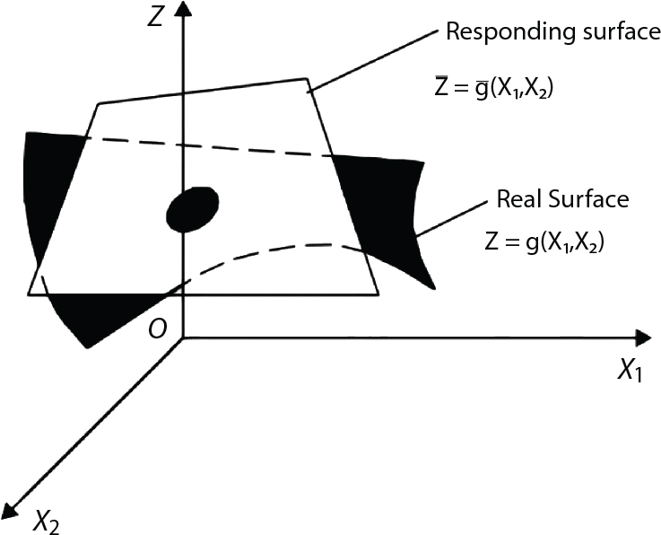
3.4 Responding Surface Method
 . There are a total of 2n+1 undetermined coefficients used to determine a, bi, ci (i=1, 2,⋯, n) on the right side of the equation. 2n+1 groups of experiments can be used to determine 2n+1 groups of responses
  . Then, the linear equations can be solved to work out a, bi, ci (i=1, 2, ⋯, n). Thus, the limit state equation of the structure can be determined.
 . Usually, the average point is taken.
 and
and  , with 2n+1 point values obtained, where f is set to 3 during the first iteration process, and then set to 1 for iterative computation.
 is substituted into step (2) for the next iteration until the set convergence accuracy is satisfied.
3.4.1 Response Surface Methodology for Least Squares Support Vector Machines (LS-SVM)
 ,
,  ,
,  ,
,  , Kji = K(xj, xi) and j, i = 1, 2, ⋯, l. Solving Equation (3.104) with the least squares method, and obtaining α and b, enables the predicted output to be obtained.
 ;
;
 ;
;
 ;
;
 , where σ, κ and θ are adjustable constants.
3.4.2 Examples
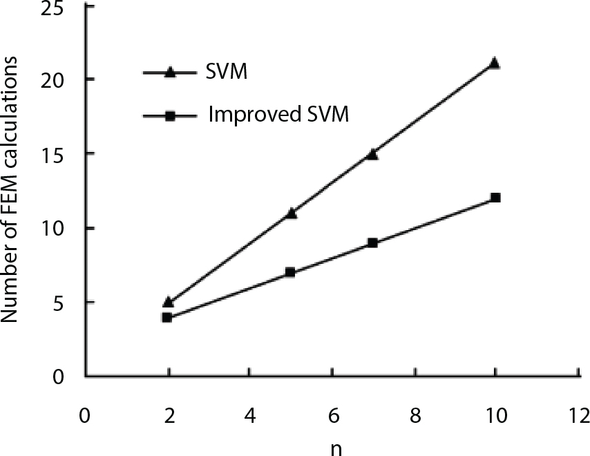
 , where the basic variable xi follows the rule of standard normal distribution. The exact solution of the reliability index for the limit state function is β=3. When n=2, 5, 7 and 10, SVM with a linear kernel function is used to reconstruct the response surface, with the reliability indexes analyzed by the SVM response surface method and the improved SVM response surface method converging to form accurate solutions. See Figure 3.4 to see how the number of FEM calculations varies with the number of variables n.
 , where x1 ∼ N(10, 22), x2 ∼ N(2.5, 0.3752).
 , where x1 ∼ N(0.6, 0.07862), x2 ∼ N(2.18, 0.06542) and x3 ∼ LN(32.8, 0.9842)
 . The random variables are the sectional areas A1 and A2 of the elements and the external load P. See Table 3.3 for the random characteristics. If the horizontal displacement u3 (unit: cm) of Node 3 is taken as the maximum deformation of the structure to be controlled, calculate its failure probability.
Examples
Calculation content
FORM method of original equation
Response surface method
Improved response surface method
Quadratic polynomial
ANN
SVM
Improved ANN
Improved SVM
Example 2-1
Reliability index
2.330
2.331
2.350
2.331
2.330
2.333
Design point
(11.186, 1.655)
(11.012, 1.647)
(11.137, 1.645)
(11.016, 1.647)
(11.183, 1.655)
(10.940, 1.643)
Iteration (times)
5
4
5
6
6
Finite element calculation (times)
29
20
26
11
11
Example 2-2
Reliability index
4.690
4.690
4.690
4.690
4.691
4.690
Design point
(0.797, 4.929)
(0.798, 4.949)
(0.794, 4.837)
(0.797, 4.931)
(0.800, 5.00)
(0.797, 4.926)
Iteration (times)
6
5
4
6
3
Finite element calculation (times)
35
25
21
11
8
Example 2-3
Reliability index
1.965
1.965
1.965
1.965
1.965
1.965
Design point
(0.46, 2.16, 33.42)
(0.46, 2.16, 33.42)
(0.46, 2.16, 33.43)
(0.46, 2.16, 33.43)
(0.46, 2.16, 33.43)
(0.46, 2.15, 33.43)
Iteration (times)
3
5
3
6
3
Finite element calculation (times)
23
35
22
13
10 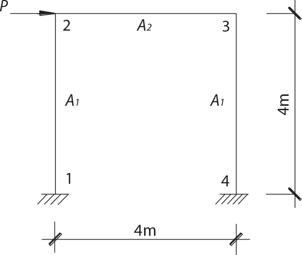
Random variables
Average mi
Standard deviation σi
Distribution type
ai
A1(m2)
0.36
0.036
Logarithmic normal
0.08333
A2(m2)
0.18
0.018
Logarithmic normal
0.16670
P(kN)
20
5
Extreme value type I
—
 . Kernel parameters σ and hyper-parameters γ exert a significant influence on the generalization performance of LS-SVM. After considering the fast solution speed of LS-SVM, the cross-validation method is used to select parameters γ and σ. The parameter set is determined for γ and σ, from which parameters are selected for combination. The LS-SVM is trained to select the best parameter combination of the model. Their generalization ability is at its best when hyper-parameter γ = 4 × 10⁸ and kernel parameter σ = 5. The estimated mean error εRMS of the learning sample and the test sample is calculated as follows:
 for the learning samples and the 10 test samples, which were all sampled according to the probability distribution of each random variable. To be specific, ε is the relative error. Due to space limitations, Table 3.4 only lists the training results of certain learning samples and test samples with relatively large errors. As shown in Table 3.4, the estimated values of the LS-SVM function of the learning samples and test samples are quite close to the results of the FEM calculation, indicating that LS-SVM can establish a correct nonlinear mapping relationship between the functions.
 . A failure probability Pf = 2.25×10⁻³, obtained by the traditional response surface method is found in the literature [3-14], while a failure probability Pf = 2.322×10⁻³ is obtained when using 2,000 iterations of the importance sampling method.
Sample no.
FEM calculation results (cm)
LS-SVM estimated value (cm)
Relative error (%)
Learning Samples
1
0.4297
0.42977
0.0159
2
0.1488
0.14878
-0.0123
3
0.1791
0.17912
0.0112
4
0.4880
0.48795
-0.0096
5
0.3371
0.33707
-0.0095
6
0.3371
0.33707
-0.0095
7
0.0753
0.075295
-0.0072
8
0.2029
0.20291
0.0053
9
0.2980
0.29799
-0.0037
10
0.54280
0.54278
-0.0031
Tested Samples
1
0.8050
0.80499
1.3336
2
0.5938
0.59382
0.9208
3
0.3694
0.36936
-0.7098
4
0.3471
0.34714
0.4757
5
0.4784
0.47835
-0.3223
 . See Table 3.5 for the sectional characteristics of each unit. The random variables are the sectional area A1 of the unit and the external load P. The statistical parameters are shown in Table 3.5.
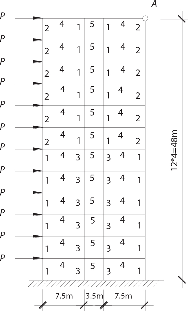
Random variables
Average mi
Standard deviation σi
Distribution type
ai
A1 (m2)
0.25
0.025
Logarithmic normal
0.08333
A2 (m2)
0.16
0.016
Logarithmic normal
0.08333
A3 (m2)
0.36
0.036
Logarithmic normal
0.08333
A4 (m2)
0.2
0.02
Logarithmic normal
0.26670
A5 (m2)
0.15
0.015
Logarithmic normal
0.20000
P (kN)
30.0
7.5
Extreme value type I
—
l
γ
σ
εRMS
Pf
Learning samples
Test samples
25
7×10⁴
9
0.051
0.3305
7.259×10⁻²
49
1.5×10⁵
11
0.0594
0.2437
7.680×10⁻²
References