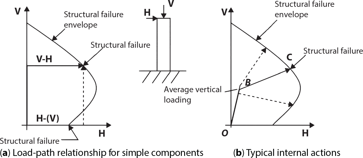
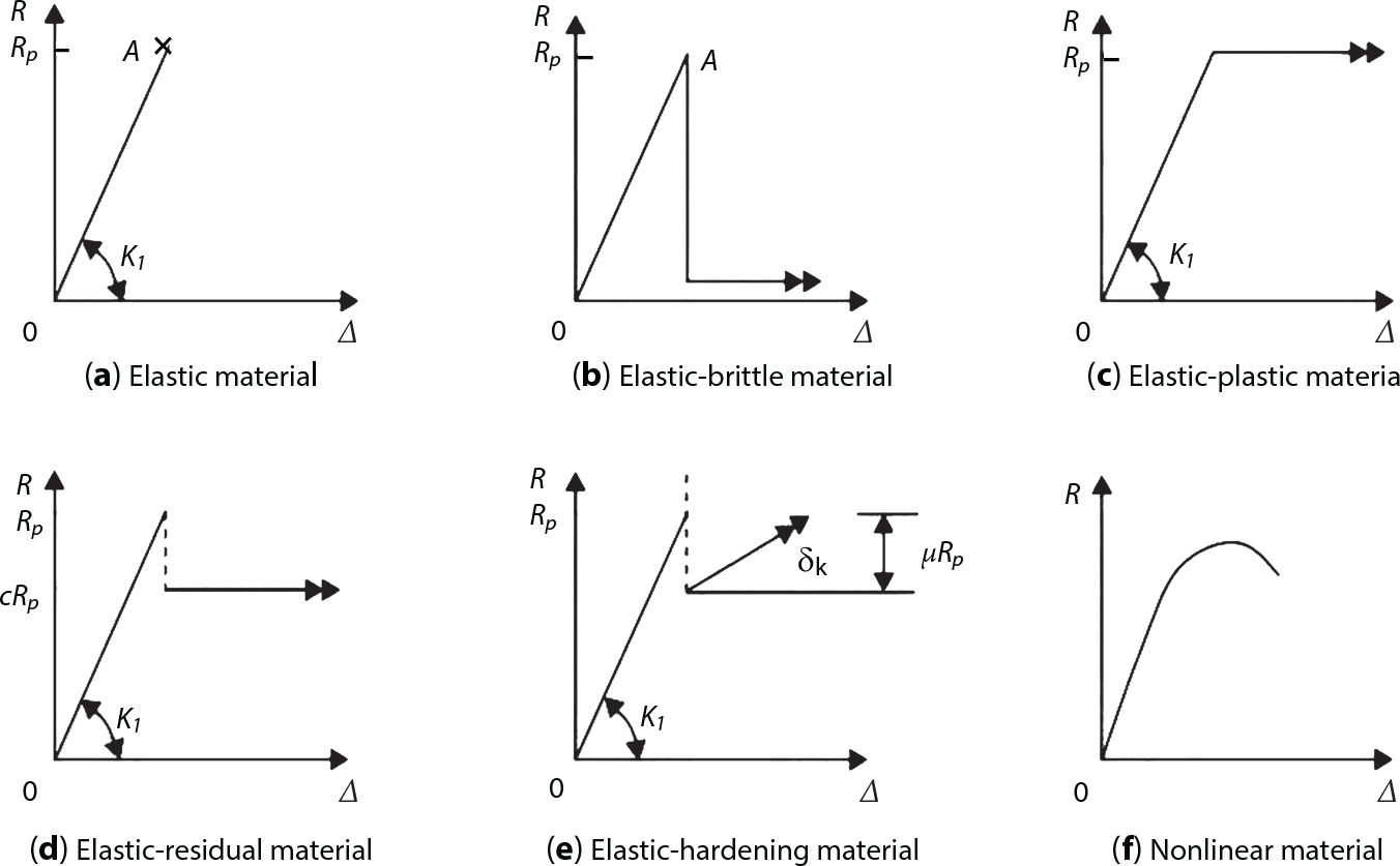
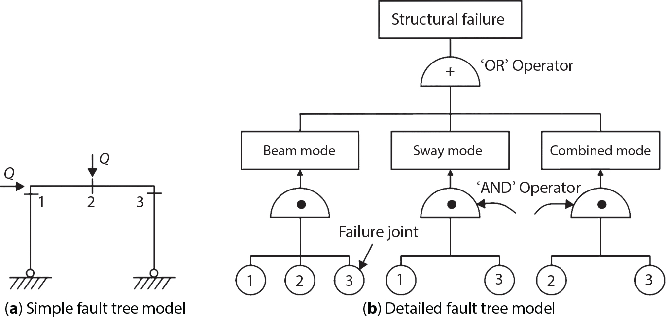
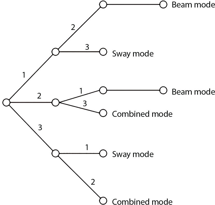
An actual engineering structure is composed of many components, and the failure of a single structural component does not necessarily cause the failure of the whole structure. Considering that the failure of a structure is marked by overall failure, the probability of overall failure is an issue related to the system reliability of the structure. It is generally believed that the key to solving the problem of system reliability lies in identifying the main failure mode of the structural system and calculating the system reliability. Usually, to identify the main failure mode of a structural system, it is necessary to repeatedly search the failure section, failure path and failure mode of the structure to generate the trunk and branches of the structural system failure tree. Therefore, in the early days, system reliability researchers focused on how to identify the main failure mode of a structural system quickly and accurately. Cornell[5-1] proposed a wide bound formula for the interval estimation method applied to system reliability calculation. Ditlevsen[5-2] proposed a narrow bound formula. Ang et al. [5-3] applied the idea of fault tree analysis to the reliability analysis of structural systems, and proposed a point estimation method, i.e., the probabilistic network evaluation technique (PNET) for system reliability analysis. With the establishment of the above theory, an available solution can be developed for system reliability analysis under the condition that the main failure modes are known. Dong [5-4] and Li [5-5] reviewed and summarized the research findings of many academic researchers on system reliability, putting forward a new method for the overall reliability analysis of engineering structures. They then explored how to use this method in engineering practice. In references [5-6] [5-7], the system reliability of offshore structures is analyzed based on the principle of most unfavorable load combinations from the perspective of engineering applications. In practice, because there are an infinite number of structural system failure modes, system reliability is difficult to calculate. The analysis of a structural system can be simplified by: (1) load modeling: the magnitude and order of applied loads; (2) system modeling: the relationship between the structural system and its components, as well as the relationship between components; and (3) material modeling: material response and strength characteristics. In addition, it is necessary to define criteria for limit state design. (1) Load simulation If the load mode of the entire structure is taken into consideration, a part of the structure will enter a (local) limit state before the whole structure reaches its limit. Therefore, the structural failure mode is likely to depend on an exact loading process. This problem is defined as a “load-path relationship”, i.e., the structural failure probability is estimated using the path generated according to the (random) vector of the loading process [5-8],[5-9]. As can be seen from Figure 5.1(a), there are two loading paths for the cylindrical specimen: the horizontal path and the vertical path. In other words, there are two loading sequences. For the structure to enter the limit state at point A, a vertical load must be applied first and then a horizontal load; if a horizontal load is applied first, the structure will fail to enter the limit state at point A. However, for actual structures, the load-path relationship is not so critical [5-10], because (1) the combined effect of internal forces at key locations causes the internal force to propagate along a path similar to OBC in (b), where OB represents the dead weight and a permanent live load path, while BC represents a limit load path; and (2) a ductile failure mode can be designed for many actual structural systems in order to avoid brittle failure, so that these structural systems are insensitive to the external loadpath. Therefore, most structures are characterized by plasticity. For this reason, the rigid plastic theory provides an approximate and accurate force analysis of structural systems [5-11]. Furthermore, the bearing capacity of a simple, ideal rigid-plastic system is not directly related to the loading path, and the failure deformation of this system is only under the control of the “orthogonal flow rule”. In the reliability analysis of structural systems, loading path-dependency is not taken into serious consideration, whereas in many practical cases, the load is idealized as a time-independent random variable. Figure 5.1 Load-path relationship. (2) Material simulation In contrast to the complexity of actual structures, material characteristics are often idealized in structural engineering practice. When structural section characteristics are considered, the relationship between components can be assumed as shown in Figure 5.2. The elastic characteristics (Figure 5.2(a)) conform to the concept of maximum allowable stress. Based on this idealized treatment, it can be considered that the failure of any part or component of a structure is consistent with the failure of the structural system. For most structures, such idealized treatment is impractical, but it is very useful. Because of structural redundancy, the brittle failure of components does not mean structural failure. Therefore, the loading characteristics of actual components can be better considered as being “elastic-brittle”. This shows that components can still deform when the bearing capacity is zero, even after reaching their final bearing capacity (Figure 5.2(b)). Elastic-plastic components (Figure 5.2(c)) allow a single structural component or specific part to continue to deform while bearing maximum stress. The structure is rigid-plastic when the stiffness Ki of elastic components is infinitely great. The elastic-brittle and elastic-plastic characteristics can be summarized as the characteristics of elastic-residual strength (Figure 5.2(d)), and further as elastic-hardening (or softening) properties (Figure 5.2(e)). The latter can be considered approximate equivalence to the overall performance, including post-buckling behavior. Even without considering the concept of reliability, it remains difficult to consider the loading characteristics of the latter in structural analysis, not to mention the analysis of the overall nonlinear (i.e., curvilinear) strength-deformation relations (Figure 5.2(f)). Figure 5.2 Different strength-deformation (R-A) relations. (3) System simulation Usually, the actual structural system needs to be simplified before it can be analyzed. For example, the centroid of the components of a frame structure needs to be idealized, the joints need to be regarded as dots, and only a few determined dots should be taken to check the strength or stress of the key sections. Similarly, the load is applied by means of nodal load or sustained load in a limited form. If the load is not a nodal load, the key points for structural safety checking may change with differing load combinations and load strength. When a structural system fails, this needs to be defined from the following different angles, since it is different from the failure of a single component or material: Structural failure modes include the combined failure effect of two or more components (or sections), such as statically indeterminate structures. The structural failure model has attracted special attention for determining the reliability of structural systems. After all failure modes of a structural system are defined, the concept of a “fault tree” can be used to systematically enumerate the failure modes (failure of components or sections) that cause failure. An example of the “fault tree” is shown in Figure 5.3 (b), corresponding to the structural component in Figure 5.3 (a). The specific process involves decomposing a structural failure mode into sub-events and then further decomposing these sub-events. The lowest sub-events on the fault tree correspond to the components or sections of the structure that have failed. A local limit stress equation can be obtained in this layer. The fault tree method is mainly used for overall reliability analysis, but it is also applicable to structural reliability analysis [5-12],[5-13],[5-14]. These methods illustrate the feasibility of simplifying a structural system, such as limiting the number of potential failure modes, i.e., the number of limit states in the structural system. For rigid-plastic structures in special cases, the traditional method for identifying failure modes is to consider the combination of the mechanical properties of the mechanism. In the reliability analysis of structural systems, different methods of system simulation can be introduced into a single element. By introducing a modeling error, we can use an idealized model (e.g., rigid-plastic stress) to simulate the actual system [5-15]. Figure 5.3 Fault tree. For the reliability analysis of a multi-component structure, there are at least two methods that complement each other, i.e., “failure” mode method and “valid” mode method [5-16]. (1) Failure mode method The failure mode method is based on identifying all potential failure modes of a structure. Each structural failure mode generally starts from the “failure” of one component after another (e.g., the components enter their corresponding limit state) until there are enough components that have failed to cause the whole structure to enter its limit state. The possible ways in which structural failure is caused can be represented by the “event tree” in Figure 5.4 or the “failure graph” in Figure 5.5. Each “branch” in the failure graph represents the failure of a structural component. Any complete path starts from the joints of the “complete structure”, involving all “failure” points and indicating the possible failure sequence of components. Such information can also be obtained from the event tree. Because the failure in any failure path may cause structural failure, “structural failure” FS is the union of all potential failure event modes: where Fi represents the ith failure mode. For each failure mode, there must be enough failing components (or failure joints of the structure). So where Fij represents the jth failing component in the ith failure mode; n represents the number of components causing the ith failure mode. Figure 5.4 Event tree of structure. Figure 5.5 Failure diagram of structure. (2) Valid mode method The valid mode method is based on identifying all states (or modes) in which the structure is valid. For the structure in Figure 5.3 (a), each joint A, B, C, D, E, F or G (except H) in the failure graph of Figure 5.5 represents a structurally valid mode (as can also be seen from Figure 5.4). For each valid mode, the structure may suffer local failure, but still retains the ability to bear loads (it is a statically indeterminate structure). For the structure to be effective, at least one valid mode is required, or where SS represents “structurally valid”; Si represents the ith structurally valid mode, i = 1…k is not equal to the final number of joints. From Equation (5.3), we get: where where Fij represents the jth failing component in the ith valid mode; lij represents the number of components causing the ith valid mode. (3) Upper limit and lower limit According to Equations (5.1) and (5.5), if all failure modes have been analyzed, pf will be underestimated when the failure mode method (Equation (5.1)) is used to estimate the failure probability of a structural system; conversely, if all the valid modes have been analyzed, pf will be overestimated when the valid mode method (Equation (5.4)) is used. For a rigid-plastic structure, a similar conclusion can be drawn according to the bound theorem of ideal plastic materials (limit analysis). Therefore, if the intensity of all loads acting on the structure is related only to one parameter, the probability that the structure suffers plastic failure {Ek} in the kth failure mode can be expressed as This represents the upper bound theorem (maneuvering conditions). In classical plastic limit analysis, the “statically determinate” method or balancing method suggests that if there is at least one statically determinate allowable stress field (i.e., the stress field is in a state of equilibrium under load, and the material does not suffer local yielding), then the structure will not fail. Now, suppose there is at least one statically determinate allowable stress field in the structure. If D means that there is no allowable stress field, then according to the theory of static determinacy, it represents a system failure. The probability of this event occurring is Prob{D} = Pϕ(w). So This represents the lower bound theorem (static conditions) in probability limit analysis. A structural system or its auxiliary system can be idealized into two kinds of systems: series systems and parallel systems. Some structural systems can be composed of these two systems, though sometimes they may be more complex. (1) Series system The series system is represented by a chain, and is known as a “weakly connected” system. The limit state of any structural component can cause structural failure (Figure 5.6). In this ideal model, the exact material properties of structural units or components do not play a critical role anymore. If a structural component is brittle, then the fracture of this component will cause structural failure; if the components have elastic deformability, then the failure may be determined by excessive yield. Thus it can be seen that a statically determinate structure comprises a train of series systems, since the failure of any subunit may lead to the failure of the whole structure. Figure 5.6 Series system. Therefore, any unit is a possible failure mode. The failure probability of a weakly connected structure composed of three units is: Compared with Equation (5.1), the series system in Equation (5.8) is a form of failure mode. If the failure mode F(i = 1, m) is represented by the limit state equation Gi(X) = 0 in the basic variable space, the basic reliability problem can be directly extended to: where Ek represents the vector form of all basic random variables (load, unit strength, unit attribute, size, etc.) and D belongs to the domain X, used to define system failure. This can be defined by several failure modes, e.g., Gi(X) ≤ 0. In two-dimensional x space, Equation (5.9) can be defined by the dashed area composed of D and Gi(X) ≤ 0 in Equation (5.7). Figure 5.7 Two-dimensional failure region for reliability problem of structural system. The safe zone is defined as where It can thus be seen that this equation is equivalent to the “valid mode” presented in the section of 5.1.2. For the chain shown in Figure 5.6, the load effect S is consistent with the load Q at every step. If FRi(r) is the cumulative distribution function (CDF) of intensity at the ith step, the CDF of the entire chain, then FRi() can be expressed as: where the strength of a single material can be converted to: This equation is the basis for the resistance probability distribution of brittle materials. When each Ri obeys normal distribution and m approaches infinity, the minimum value of R obeys Extreme value type III distribution. For the series system model, the failure of one component causes redistribution of the internal force and leads to the failure of another component, and so on. Therefore, the failure probability of the whole structural system can be approximated to the failure probability of the first set of (brittle) components [5-17]. However, when there are many redundant brittle components, this approximation method is not applicable, because the residual strength becomes critical. (2) Parallel system When the elements of a structural system (or subsystem) are interconnected in such a way that one or more elements can enter a limit state without there being an important effect exerted on the failure of the whole system, then such a system is called a parallel system, or a redundant system. Figure 5.8 shows two simple parallel systems. There are two forms of system redundancy. When the redundancy unit plays a role as soon as the structure is subjected to a small load, we call this “active redundancy”. If the redundancy unit does not start functioning until a certain number of structural units fail or degenerate, we call this “negative redundancy”. This shows that the redundancy unit increases system reliability. Whether active redundancy is helpful or not depends on the characteristics and failure definition of components or units. For an ideal plastic system, the “static theory” ensures that active redundancy does not reduce the reliability of the structural system [5-17]. Under the action of active redundancy, the failure probability of a parallel (sub-) system composed of three units can be expressed as: where Fi represents the failure probability of the ith structural component. Thus, it can be directly determined that Equation (5.14) is equivalent to Equation (5.4) and can be expressed in X space as: Figure 5.8 Two simple parallel systems. In contrast to the series system, the parallel system will not fail unless all the active components enter their respective limit states. This means that the performance of system components is very important to the definition of system failure. (3) Parallel system For ideal plastic materials in the perfect plasticity, there are totally different. Taking a steel frame structure as an example (Figure 5.8(b)), the failure of each component can be expressed by the following equation: where Qi(i = 1, …) represents external load; Δi represents the deflection relative to Qi (as a function of θj and size); Mj represents the plastic resisting moment at j = 1, …; θj represents the plastic rotation angle at j = 1, …. Equation (5.16) clearly reflects this parallel system, because all Mj can be superimposed together to resist external load Qi. A series system comprises a set of failure modes consisting of a single failure equation like Equation (5.16). This is because structural failure is bound to occur when any failure (or collapse) mode occurs. Thus, there may be more than one failure mode of plastic bending moment in the system, indicating that there may be no difference in the structural bearing capacity obtained from different failure modes. (4) Conditional combination system A complete system is usually composed of several series and parallel subsystems so that it can realize its function. The connection between components and the failure mode of subsystems have an important impact on the limit state of the whole structure. For a complex structure, this is not a simple exercise. Not only will the structural internal force be redistributed after the failure of components, but loads will also change with structural response over time (structural deflection). An actual structural system model may also require the use of a conditional system or its subsystem. If the failure of an individual unit or a group of units affects the failure of other units or groups of units, then the latter will suffer associated failure. For example, if the top beam collapses in Figure 5.9, this may affect the performance and reliability of the bottom beam (because the bottom beam may be destroyed and come under additional load). In this case, the possibility of structural unit failure depends on the performance of the structure in extreme conditions. If the sequence of events can be enumerated, then the structure in a conditional event can apparently be reduced to a group of units or subsystems that contain both “series” and “parallel” components. Therefore, the complex system can be decomposed into several subsystems or subunits to constitute the evaluation process of system reliability. Jin [5-6][5-7] proposed a simplified model considering pipe-pile-soil interaction, and used it to evaluate the reliability of the jacket platform system. In this case, the jacket platform system was divided into three subunits: jacket structure, pile and soil. The failure probability of each subunit in the given load mode was calculated, and the reliability of the whole structure system calculated according to the failure mode of the series system. During the evaluation of system reliability, the nonlinear push-over structural analysis method and importance sampling method were used to calculate the reliability of the jacket platform system. Figure 5.9 Condition system. Similar to component reliability, structural system reliability can also be calculated using the immediate integration method. However, there is an alternative method, by which upper and lower bounds are established for failure probability of the structural system for analysis. It is assumed that a certain structural system, undergoing a series of loads, may fail in any possible failure mode under the action of any load. So, the total probability of structural failure can be expressed by the failure probability in this mode: where Fi represents “structural failure in the ith mode under the action of all loads”; Si represents “structural survival in the ith mode under the action of all loads (i.e., survival rate of structure). These are complementary events. So It can be written in the following form: where (1) Linear series system The probability of structural failure can be expressed as P(F) = 1 − P(S), where P(S) represents the probability of structural survival. For mutually independent failure modes, P(S) can be expressed by the probability of survival in each mode, or directly by where When all failure modes are completely correlated with one another, the weakest failure mode is the most likely to directly cause structural failure when the contingency of material strength is ignored. So Equations (5.19) or (5.20) and (5.21) can be used to define a relatively rough boundary for the failure probability of a structural system when any failure mode is completely independent from or completely correlated with the rest: However, for most engineering structure systems, the boundary set Equation (5.23) is too large to be practical. (2) Quadratic series boundary The quadratic series boundary can be obtained by maintaining the form of Because the number of the terms that are alternatively positive and negative increases with the number of terms in the equation, the upper bound of P(F) can be obtained by considering the linear conditions only (e.g., P(F1)). The lower bound can be obtained by considering the linear and quadratic failure conditions only. The upper bound can be obtained by considering the linear, quadratic and cubic failure conditions, and so on. It should be noted that the probability of structural failure cannot be reduced if an additional failure mode is considered. Therefore, every complete row in Equation (5.24) has a non-negative effect on In these two forms, the results depend on the sequence of the marked failure modes. Operation rules [5-20] are established for an optimal sequence of events in order to obtain an optimal boundary. By means of an effective rule we can sort modes from high to low in the order of their importance. For a given sequence, a more rational boundary can be obtained by using Equation (5.25) than by Equation (5.26); if all possible sequences are considered, then the boundaries obtained by these two equations will be consistent with each other [5-21]. An upper boundary can be obtained by simplifying each line in Equation (5.24). As pointed out above, a standard line, such as the fifth line, has a non-negative effect on With P5 removed, the other lines can be written as: where Eij represents event ij. For any events, A and B, if Since V5 has a non-negative effect on U5, boundary Equation (5.29) will increase the right boundary value of Equation (5.28). So However, because Pj5 = P(Fj ∩ F5), and since the fifth line is a typical line, it satisfies: This result may also depend on the sequence of failure events. The calculated results of Equations (5.29) and (5.31) with respect to rigid and rigid-plastic frames have been compared with the results of Monte-Carlo simulation [5-22]. In a certain distribution form and within a certain variation range, the boundary obtained by calculation is generally quite close to the simulation results. However, they are not always close to each other. (3) Quadratic series boundary under sequential loads Load sequence and correlation determine the failure probability boundary of systems. According to Equation (5.17), under load vector Q1, Q2, Q3…, the probability of structural failure can be expressed as: where Fi represents “structural failure that occurs under the action of the ith load”; S means that “the structure is valid under the action of the ith load. They are complementary events, In general, failure under the action of the ith load is correlated with survival before the application of the ith load. The equation below can express this “transfer” of probability: Moreover, because Similarly, for other parts consistent with Equation (5.17), by using Equation (5.32), P(F) can be expressed as: Or, for the application of n sequential loads, we obtain: The above equation is consistent with Equation (5.24), where (4) Series boundaries and sequential loads in multiple modes The boundary Equations (5.25) and (5.31) of failure modes can be summarized as failures in multiple modes within the range of load sequence. Equations (5.25) and (5.31) can be interpreted as the probability In practice, Fi, Fj are usually related to each other, making it difficult to work out Similarly, if events Fi, Fj are completely related to each other, and the critical state is known, then where When it is known that load sequence and multiple failure modes are independent of each other, then the maximum value of the terms on the left side can be replaced by the summation formula; similarly, if the load sequence is known to be completely correlated with multiple failure modes, then the summation formula for the terms on the right side can be replaced by the maximum value. If the composition N of load sequence is known to be continuous, and there is a shared probability density function (PDF) for the alternating independent loads, then the right boundary can be replaced by the following formula: (5) Optimization of series boundaries and parallel system failure boundaries If the results of quadratic series boundaries gradually deteriorate when (linear) LSF dependency increases, the problem can be transformed into a low-dependency LSF for boundary optimization. Alternatively, if higher-order parts can be preserved, the boundary of the series system can be optimized. For example, if in where is In addition, the sequence of some failure events is of great significance for obtaining an optimal boundary. However, it is most difficult to estimate Pijk, since it is jointly affected by all three parts. When the event Fi is expressed as a linear function, the nonlinear lower limit can be obtained from the following equation [5-24]: It is known that ρkj > ρjk ρij > 0, where ρij is the correlation coefficient of the linear failure function for events i, j. Feng [5-25] has proposed a good method for solving Pij and Pijk in linear LSF. For the failure probability of parallel systems, it can be calculated by Equation (5.2) or Equation (5.14). For this kind of boundary, it can be created by applying series boundaries to the terms on the right side of the identical equation: The boundary value obtained by the above equation is low, since for a highly reliable system, the second term on the right side of the equation is close to 1.0. Dependency can also enhance load dependence, in particular the dependence between the load and a single structural component [5-26] [5-27]. The correlation between basic variables in second-order reliability analysis is determined by transforming the correlation set into a non-correlation set. Two static loads are applied simultaneously to the correlation effect of rigid-plastic portal frames, and the set of its typical results is shown in Figure 5.10 [5-28]. However, there is a lack of actual experimental data on the dependence between intensity (and load). In general, a conservative assumption needs to be put forward. Figure 5.10 The impact of correlation on system security indications. In practical applications, it may not be possible to express the limit state surface explicitly by one or more implicit limit equations, while it is often implicitly understood in the process of finite element analysis. G(X) is used to represent the structural response, and G(X) is the implicit function of random variable X. When calculating G(X), let The discrete points can be fitted to determine the order of n in the polynomial, and the results will affect the number of evaluations and the number of estimated derivatives. Also, for a well-conditioned system of equations, If an actual limit state equation is established by the results of discretization only, it will be impossible to obtain its form and order, let alone estimate its design point. This means that there will be no guidance on the selection of the estimation function where The (regression) coefficients can be obtained by a series of simulation “experiments”, i.e., a series of structural analyses can be conducted by inputting selection variables depending on the “experimental design”. For approximate experimental design, it is necessary to consider the reasonable and accurate estimation of failure possibility. This shows that the focus needs to be on the maximum probability area, including the failure zone, i.e., the design point. However, as mentioned above, this is unknown at first. Therefore, a value near the average variable can be selected as an input variable for experimental design. A simple experimental design is shown in Figure 5.11. Rajashekhar and Ellingwood [5-33] have discussed more complex problems. Once the experimental design is selected and the equation G(X) is calculated, it can be seen that there is an error between the actual value of Figure 5.11 Simple experimental design of two variables. Let vector D represent the regression coefficients A, B, C. In this case, Equation (5.42) can be expressed as G(D, X). Similarly, for each point (1) Simplification of large-scale system For some practical problems, it is impractical to apply Equation (5.42) because there are too many variables. For example, this will happen when finite element analysis (FEA) is adopted for structural response. Therefore, the number of random variables involved can be reduced in many ways. The first way is to replace free variables with formulas for determining uncertainty. The second way is to reduce the set of random variables, X, to the minimum set, XA, while describing their mean spatial value. For example, we can use the same (e.g., spatial averaging) yield strength at each point in the stress plane, rather than exactly representing different yield strengths from point to point (or from finite element to finite element). The third way is to simplify the error effect of random variables (or spatial averages), i.e., they may contain only a single additional effect to response, rather than a more complex relationship. In this way, we can establish an Equation (5.44) for the additional error effect: where ej, ejk, … represents the error term caused by spatial averaging (it is assumed that spatially averaged random variables are independent here), and ε represents the retained error (e.g., those caused by the degree of freedom). If ej, ejk, … can be obtained separately, this form is useful, e.g., by analyzing the change of the spatial averaging effect. The error can be fitted by G(X), and ε can be restricted. (2) Iterative solution method The optimum fitting point between the approximate responding surface and the actual (non-explicit) LSF is uncertain in advance. It has been suggested that these points can be determined by iterative search. Let Equation (5.42) contain sufficient undetermined coefficients to accurately estimate If Xm is a design point, other points can be found on the approximate surface The speed of this calculation method, which also boasts high fitting accuracy, is related to the selection of the design point and the shape of the actual (non-explicit) LSF in the search area. Obviously, when the design point representing resistance is on the left truncated section of this random variable, while the design point representing load is on the right, the calculation results will be improved [5-34]. Moreover, in general we cannot ensure that all possibly related design points converge. It is possible to modify the search algorithm so that the search deviates from the design points included. (3) Responding surface and finite element analysis The responding surface is not a method explicitly required for reliability analysis. When FORM is used, we suggest taking the responding surface as a tool to apply FEA to structural reliability analysis. It should be noted now that in standard normal space, the quadratic responding surface is essentially similar to the second-order second-moment theory. This is because a quadratic surface can be used to fit either a known nonlinear limit state surface or a known discrete point on the responding surface. The result is that these two methods feature extremely similar discussions. When the responding surface method is used for FEA, the repeated results contain a series of selected points determined by the finite element program, such as those [5-35] that apply to the responding surface. If FORM is used, the fitted surface is linear, and only a small number of points are required to determine the responding surface. This is because, generally speaking, the fitting of the responding surface has nothing to do with the reliability calculation. One requirement is that the gradient of the design point should be determined or estimated. Some FEA programs can be modified to meet this requirement. Alternatively, an approximate finite difference method can be adopted, but this will come with a higher calculation cost. However, the responding surface method has been combined with FORM in some commercial finite-element codes [5-36]. Importantly, the finite element model represents a random field in a reliability environment, e.g., statistical variables that may be required to represent performance, such as cross-plate Young’s modulus. This is quite a specialized topic, and many methods have been proposed [5-37][5-38][5-39][5-40]. (1) Truncation enumeration method For a complex structural system, the best way to determine all structural failure modes is to enumerate all combinations of joint failure. This is a huge amount of work, as all the sequential probability of joint failure needs to be considered. All joints are analyzed in turn and then added to the sequence of joints that failed previously. Every new sequence can be checked to find out whether a feasible system failure mode has been obtained. If not, more joints will be added to the sequence. If structural failure is identified as a collapse, then the failure mode must be kinematically feasible. When a failure mode is identified, we can enumerate the next failure mode by tracing back until a new joint combination appears, as shown in Figure 5.12. Figure 5.12 Systematic enumeration process. If those failure modes that have a small probability effect on the system can be identified, then the calculation will be greatly simplified. If the error is insignificant, it can be eliminated from subsequent calculations [5-41]. Obviously, it will be advantageous if this can be done at the early stage of enumeration, preferably before the mode failure probability is calculated. Many techniques have been proposed[5-42] [5-43] [5-44] [5-45] [5-46] [5-47], with some more intuitive than others. One rational technique known as “truncated enumeration” will be described below. Because all failure modes have been determined, it is not important to reveal their order. So, for the convenience of enumeration, structural elastic stress analysis should be performed. Of course, the specific order of failure modes obtained depends on the enumeration method used. After specific modes have been eliminated, this order will have an impact on the calculation of failure probability. For elastic and rigid-plastic joints, structural behavior is generally quite similar. Moreover, for rigid-plastic behavior, the failure mode and corresponding stress field are irrelevant to the elastic properties of any such structure. In an order containing n joints, the probability of the kth joint can be calculated as follows: where Ei represents the “resistance breakthrough of the ith joint” in the event. As shown by 1, 2 and 3 in Figure 5.12, there are many such modes in existence. The number n of joints required for structural failure depends on the criteria for structural failure judgment. For structural failure, n must be large enough to find a feasible failure mode. If pjk ≤ δPf for all modes, then the number of failure modes to be considered will be reduced. Here, δ is an appropriate “truncation criterion”, and Pf represents the estimated failure probability of the nominal structural system. Apparently, if δ = 0, it will be exhaustive. Unless objective estimation has been carried out before analysis, it may be possible for Pf to be obtained from the currently known maximum Pf value. For example, in the previous estimation, the mode failure probability is the current value, defined as Apparently, For any diversity of Equation (5.48), q ≤ n, the truncation condition Theoretically, a joint sequence can be selected in any order. However, for an efficient algorithm, the joint with the greatest contribution must be selected as soon as possible. As a result, the estimated value of Pf in Equation (5.47) will be optimized, and therefore, trivial modes will be removed as early as possible. A reasonable way is to select the next joint, so that the probability of occurrence of some joint sequences, including selected joints, can be maximized. From the first joint to the qth joint, this means that joint selection is: The first joint: The second joint: Or in general, for the qth joint: Maximization is applicable for all “eligible joints” at the level of selection (see Figure 5.12). Therefore, at the qth layer, events E1 ∼ Eq−1 are fixed, and a decision can be made to select event Eq according to the remaining joints. The simplification of Equation (5.49) helps to save time. For Equation (5.49c), approximation is suggested to cover the upper limits: These are called “one-dimensional” and “two-dimensional” branch conditions, respectively. For example, Equation (5.50a) can be interpreted physically as follows: It is practical to select the joint with the maximum failure probability rather than determine the maximum probability of occurrence by searching the entire sequence. It does not need to be the same as Equation (5.49), for the reason, when there is no difference in stress distribution at each joint, there is correlation among events E1, E2, …, Eq. For any level q, the mode failure probability conservatively estimated (overestimated) in Equation (5.48) may be conservatively estimated (overestimated) again in Equation (5.50b). Since Equation (5.50b) is now already overestimated, Equation (5.47) may also be overestimated. Therefore, some modes may be unreasonably excluded from the truncation criteria. However, these modes don’t have to be important unless they have a failure probability like For the truncated enumeration method, it is necessary to establish the sequence of joint failure events and calculate their probability. This requires the structural stress to be analyzed in steps. Once various system failure modes have been determined, a limit state equation can be established for structural failure. Two analysis processes are proposed in order to establish the limit state equation. It is assumed in both cases that the failure sequence of joints is known, and that the failure mode is the kth mode. (1) Joint substitution (“simulated load”) method In this method, the failure joint is replaced by its resistance after failure. For all subsequent external load increments, this resistance can be considered as a locally applied simulated load, whose random characteristics are the same as those of the resistance after failure [5-47]. Therefore, if the joint is fully plastic, the plastic resistance can be applied as a simulated “load”; if it is elastic-brittle and there is no brittle strength, no simulated “load” will be applied. Apparently, with the increase of external load, it is necessary to seriously check the stress state of all joints. Although this method looks outstanding, there is still a lack of proper judgment criteria to make it work. (2) Incremental loading method If the components show elastic-plasticity, and there is a known failure model k, then the failure probability can be obtained by comparing the system resistance RS with the single-parameter loading system Q1: In case of structural failure, the system resistance can always be expressed as the maximum of all accumulated load increments: where rj represents the jth load increment related to the mode failure event Ej. Therefore, a structure in which three components must fail before structural failure, r1 represents the load when the first component has failed (starting from 0), r1 + r2 represents the total load when the second component has failed, r1 + r2 + r3 represents the total load when all three components have failed. Considering that the load may disappear after a component fails, the structural resistance RS is expressed by the maximum load, i.e., Equation (5.52). The corresponding probability of failure (kth) is: It can also be expressed as: The system resistance R is controlled by the nodal force, which can be related to the load increment rj through a matrix equation: where Equation (5.55) can be extended to be suitable for more generalized joint stress behavior, such as elastic unloading strain hardening, or for more than one load system (each model serves as a random variable and each one is applied only once) where B is an “unloading matrix” related to the unloading part corresponding to deformation; CQ represents the random action of components under (no increment), and Ar is defined by Equation (5.55). It should be obvious that any load system can be chosen to determine the load increment system for load increment r. The incremental process has no other purpose, because the order of joint failure is known, causing it to be canceled out. Unloading and strain hardening (or post-buckling) behavior bring about various limitations and problems in the deterministic analysis of (incremental) structural reliability. Therefore, it is necessary to consider the range of the hardened zone, the possible reversal stress and concomitant change of local rigidity in incremental analysis. (3) Possibility estimation of system To calculate the (nominal) failure probability of the structural system, we must also calculate the failure probability of each dominant failure mode by Equation (5.57), as follows: as well as the series combination of pfk. These calculations are usually different from those for branch selection and truncation unless the probabilities have been precisely determined (in this case, it is necessary to consider the possibility of correlation effects). If the probability of the dominant mode is known, then the nominal failure probability of the structural system can be calculated theoretically by means of Equation (5.1) where Fi = (i = 1, …, m) represents failure in the ith mode. If only the dominant mode is considered, a small probability will be underestimated (see Section 5.2.2). There is an upper limit for the error introduced into the estimation of probability through truncated (i.e., abandoned) failure modes. It can be obtained by estimating the probability related to the unbranched joints at the first layer [5-48]: Although the truncated enumeration method is commonly applicable to single load parameters or single loads (i.e., time-independent cases), and is useful for determining failure modes [5-49], in general, it (and other similar methods) requires a lot of calculation. Fortunately, for common ideal rigid-plastic structures, there are alternative methods for determining failure modes. Sigurdsson [5-50] proposed to use joints in place of (artificial loads) (but not by truncation) for system reliability analysis to calculate rigid-plastic structures. For rigid-plastic joints only, Murotsu et al. [5-51] and Thoft-Christensen and Sorensen [5-50] have proposed applicable calculation steps similar to the truncated enumeration method. The research on the overall reliability of traditional structures remains limited to the scope of framed structures, i.e., it is still under the limits of ideal elastic-plasticity. For complex structures composed of plates, walls, blocks, etc., as well as for other common nonlinear physical problems, the above methods are basically unusable. For traditional analysis of overall structural reliability, problems are studied from a phenomenological perspective according to the consequences of failure. Therefore, it is essentially unable to reflect the real physical development process of the structural state from linear to nonlinear. Although nonlinear structural analysis is performed during the above-mentioned process for the branch-and-bound method, the position and failure path of plastic hinges cannot be determined yet due to randomness. Thus, structural failure and failure path must be physical processes “modified by probability” rather than real physical processes. This error in analytical methodology is the fundamental cause for the secular stagnation of traditional research on overall reliability. Correct research should be based on an analysis of the structural stress process and an investigation on the law of propagation of randomness within the physical system. For the comprehensive physical method, probability dissipation conditions need to be established for generalized probability density evolution equations in accordance with physical criteria. That is, for a given failure limit, The representative point up is a point at which the overall state of the structure is observed. It can be flexibly selected according to the object of specific analysis. For example, the fixed-point displacement of a structure can be used for a high-rise building. The reliability analysis of a structural system is the same as that of its components, but it is necessary to consider multiple failure paths related to the structural system and their corresponding limit states. For other methods, it is beneficial to connect systems in series or in parallel, or to classify more complex subsystems, e.g., the system reliability boundary theory can be used in combination with FORM. Structural failure modes are not always known. To some extent, they can be tested by Monte-Carlo simulation, by the method of exhaustion or by other simplified methods. Among these, the failure mode method, which contributes the most to failure probability, is of special concern. As mentioned above, all the methods discussed in this chapter have limitations on structural loads. Proportioned (i.e., single load parameter) loading conditions are equivalent to the problem of reliability arising under a single ultimate load (i.e., the maximum load that can be borne by the system during its service life). For a complex structure, the critical limit state may change with a sequence of multiple loads. In this case, the system itself depends on the loading path. It should be noted that, although there have already been many studies carried out on this problem, there is as yet no widely accepted method. A practical way is to define the combination of loads in reliability analysis as being like the one used for traditional structural design, i.e., only a limited number of load combinations are considered [5-15]. Although it is not a fundamental approach, this method can at least be used to analyze conditional probability under clearly defined conditions. The comprehensive physical method can better solve the problem of reliability. The offshore jacket platform is a pile platform supported by piles driven into the seabed. It can be divided into group pile type, pile foundation type and leg pile type, and is composed of a jacket, a pile, a jacket cap and a deck [5-52]. Cazzulo [5-53] studied the reliability of pile foundation structures for offshore jacket platforms, substituting the pile foundation analysis results as input conditions into the reliability analysis of the structural system. Amdahl [5-54] studied the final bearing capacity of jack-up offshore platforms with a foundation effect. Hamse [5-55] used the stiffness matrix for pile heads to describe the influence of pile-soil interaction on offshore jacket platforms. However, these methods do not consider the pile foundation and superstructure, but adopt a simplified analysis method to deal with it, which involves a certain amount of approximation. Therefore, if the pile-foundation offshore platform system can be taken, while considering both the pile-soil interaction and the influence on the offshore platform structure, the final bearing capacity of the entire system can be studied. Moreover, considering the discreteness of soil parameters, this research will become very meaningful for studying the range of influence and mode of action of soil parameters on the bearing capacity and reliability of an offshore platform system. (1) Pile-soil calculation model The final bearing capacity of a single pile under vertical load is composed of the friction force Qf of the pile body, and the supporting force Qp of the pile end, where: Where: As and Aq are the surface area of the pile body and the gross area of the pile end, respectively; f is the surface friction force per unit area. For cohesive soil, f can be expressed by Olson’s calculation [5-56]: For sandy soil, there will be Where: Su is to describe the shear strength of cohesive soil, the effective covering pressure of soil at the calculation point; K is the lateral earth pressure coefficient, the internal friction angle of sandy soil, and Q is the bearing capacity of unit pile end; Nc and Nq are dimensionless bearing capacity coefficients for cohesive soil and sandy soil, respectively. Considering the transfer of a pile under an axial load and the displacement of a pile, Kraft [5-56] put forward the axial load transfer curve of a pile based on practical experience and a full-scale pile loading test. As shown in Figure 5.13 and Figure 5.14, t is the bond between dynamic pile and soil, tmax = f, Q is the bearing capacity of the dynamic pile end, D is the outer diameter of the pile, and z is the local displacement of the pile. The final bearing capacity of soil to pile under a lateral load can be determined based on the resistance of soft cohesive soil, hard cohesive soil and sandy soil. The expression for resistance of soft cohesive soil under a shortterm static load is as follows: Figure 5.13 t ∼ z curve. Figure 5.14 Q ∼ Z curve. Where J is a dimensionless empirical coefficient between 0.25 and 0.50, which can be determined by field testing, and x is the depth of soil layer at the calculation point; for hard cohesive soil, this becomes: The load-displacement (p-y) curves for the two cohesive soils are shown in Figure 5.15a and Figure 5.15b, where y50 is the displacement value corresponding to the strain value, that is, y50 = 2.5ε50 D, ε50 it is the strain that occurs at 50% of maximum stress in an undrained test for undisturbed soil. Figure 5.15 P-y curve of soil. The resistance of sandy soil under a short-term load can be expressed by the following formula [5-57] And The Equation (5.68a) is suitable for shallow soil, while the Equation (5.68b) is suitable for deep soil; where K is the initial modulus of the soil. The calculation model for pilesoil interaction can therefore be determined using the foundation reaction coefficient method. Figure 5.17 shows the model for calculating the reaction coefficient at each point on the pile, which uses the τ ∼ z curve of Figure 5.13, the Q ∼ z curve of Figure 5.14, the p-y curve of Figure 5.15, and Figure 5.16 the expression described in Equation (5.68). In the model shown in Figure 5.17, the distortion of the pile and the deformation of the rotation angle are ignored, which is acceptable in most practical application. Figure 5.16 p-y curve of sandy soil. (2) Uncertainty of soil The strength and stiffness characteristics for each layer of soil samples used here are shown in Table 5.1. Due to the discreteness of the soil samples, the layer properties listed in Table 5.1 reflect the average value of the measured data, but in practice they show great variability. The reasons for this uncertainty of soil properties include soil classification, soil sampling, soil testing methods and calculation models, which are manifested as statistical uncertainty, testing uncertainty and knowledge uncertainty. The former two are mainly used for soil parameters, while the latter comes from the calculation model for soil, which includes the formulas for calculating axial tension (compression) pile, lateral load pile and pile tip bearing capacity. Referring to AP2A-LRFD [5-56] and the Beihai site data [5-57], Table 5.2 gives the deviation, coefficient of variation and probability distribution characteristics of various soil parameters, while Table 5.3 shows the uncertainty of the soil calculation model, which will be used as the basis for probability analysis of pile bearing capacity. Figure 5.17 Calculation model of pile. The single pile selected here has a diameter of φ2438 and a pile length of 60m, and is buried in the calculated soil as shown in Table 5.2. The pile is divided into an average of 40 finite elements, with each joint comprising two horizontal nonlinear spring supports and one vertical nonlinear spring support (see Figure 5.17). The stiffness of the nonlinear spring can be determined using the pile-soil interaction model described in the previous section, while the bearing capacity of a single pile can be calculated using the nonlinear progressive failure analysis method. As a comparison, the mean value of each variable is selected for calculation during the deterministic bearing capacity analysis of a single pile, while 500 random samples are generated for each variable during the probabilistic bearing capacity analysis. Every nonlinear progressive failure analysis includes three load conditions, namely axial tension load, axial compression load and lateral load. Table 5.1 Soil parameters. Table 5.2 Uncertainty of soil parameters. Table 5.3 Understanding the soil calculation model. Figure 5.18 Load-bearing capacity under axial compression. Table 5.4 shows the deterministic analysis results and the statistical results of the probability analysis on the bearing capacity of a single pile under axial and lateral loads, where Δ represents the bearing capacity under lateral displacement of the pile top. Figure 5.19 shows the load-bearing capacity under axial compression and tension, respectively, as well as the probability distribution simulation for load-carrying capacity. The lateral bearing capacity of a pile top under fixed end and hinge constraints is shown in Figure 5.20. Table 5.4 Bearing capacity of a single pile. Figure 5.19 Load-bearing capacity under axial tension. From the above analysis of the single pile bearing capacity, it can be seen that: (1) for large diameter piles, the effect of pile tip bearing capacity is significant. However, when the ratio of pile length to pile diameter is greater than 20, the effect of length can be ignored. (2) The ratio of axial tensile bearing capacity to compressive bearing capacity of a pile is 0.30, which means that when the upper vertical load of the structure is small, especially for a tripod jacket, structural volume damage may result from the axial tensile bearing capacity of the pile. (3) The uncertainty of axial bearing capacity distribution of a single pile due to probability analysis mainly comes from the uncertainty of the pile-soil calculation model; the coefficient of variation of the axial tension pile is 0.20, which is greater than the 0.17 of the axial compression pile. (4) The axial bearing capacity of a single pile obtained by deterministic analysis is very close to the mean value obtained by probability analysis; the probability distribution of the axial tensile bearing capacity obeys lognormal distribution (see Figure 5.19), while the axial compressive bearing capacity obeys normal distribution (see Figure 5.18). (5) The determination of lateral bearing capacity of a single pile is related to the constraint conditions of the pile head. The bearing capacity of articulated constraint of the pile head is only about 50% of that of the fixed end constraint, but the actual constraint of the pile head lies between the fixed end and the articulated end. (6) The average value of lateral bearing capacity of a single pile obtained by probability analysis is about 0.96 of that obtained by deterministic analysis, but its coefficient of variation is small and obeys lognormal distribution (see Figure 5.20). Figure 5.20 Lateral bearing capacity with different pile top constraints. (1) Structural model A tripod jacket platform is selected as the type of structure, as shown in Figure 5.21. The platform is in an ocean area with a water depth of 70m, and supported by three piles with a pile length of 60m; as a result, the main form of load it needs to bear is wave loads. Depending on the direction of wave incidence and the possibility of combination with other loads, there are a total of 8 calculation conditions for the structural system [5-57]. The entire platform structure can be discretized by the finite element method, for which the jacket structure has 29 nodes and 78 beam elements, and the pile foundation has 93 pile nodes, 90 beam elements and 96 spatial nonlinear spring elements. The pile-soil interaction is simulated by means of a nonlinear spring element and calculated using NLSPRINT software. The load-bearing capacity of the whole offshore platform system is calculated by nonlinear progressive failure analysis. This method enables the calculation of deformation and mechanical properties of the offshore platform in various states under given load conditions, reflecting the non-linear material and geometric characteristics of the structure and the final bearing capacity. Figure 5.21 Deterministic analysis of computational structure model. To analyze the influence of the structure-pile-soil interaction on an offshore platform structure, three kinds of supporting boundary conditions are considered during bearing capacity analysis. These are the fixed end support at the mud surface line, the linear spring at the mud surface line (to consider the effect of soil action), and the pile support (to consider the nonlinear effect of the pile-soil). The stiffness of the linear spring at the mud surface line is determined by the displacement caused by a unit force acting on the pile top. Figure 5.22 Shear and bending bearing capacity and structural placement diagram. (2) Bearing capacity of pile foundation The final bearing capacity (shear bearing capacity) of an offshore platform structure under an environmental load is shown in Figure 5.20, with the shear and flexural bearing capacity and structural load-displacement curve under operating condition 1 shown in Figure 5.22. It can be seen that: (1) For a jacket platform structure, the influence of the supporting boundary conditions on the bearing capacity of the structural system is significant. The bearing capacity of an offshore platform structure with fixed end support is slightly greater than that of a linear support on a mud surface, but significantly greater than that of a nonlinear spring support. For both linear and nonlinear spring supports, the displacement value corresponding to the maximum bearing capacity will be greater than that of the fixed end support. (2) In terms of the failure state of the structure, the failure of the structure with a nonlinear spring support is mainly composed of the bearing capacity of the pile foundation, that is, the axial tensile failure of the pile can also show changes in stress and strain in the process of reaching the final bearing capacity of the structure. In contrast, the consolidated structure on the mud surface or linear spring support is composed of the compressive buckling or joint failure of the members of the structure itself. This shows that the analysis method for bearing capacity of an offshore platform structure with linear spring support is able to consider the influence of the structure-pile-soil interaction. (3) Because of the effect of soil, the bearing capacity of the structure supported by a fixed end is approximately equal to that of the structure supported by a linear spring, which is only manifested in the difference of structural displacement. For the structure supported by a nonlinear spring, the stiffness of the spring changes with every load, which absorbs the energy generated by an external load and leads to an increase in structural displacement and a decrease in bearing capacity. This shows that, if the bearing capacity of the whole offshore platform structure can be improved, it will be necessary to coordinate the bearing capacity of the pile foundation and structure. (3) Probability analysis According to the deterministic analysis results of the bearing capacity of the offshore platform structure system, and to better study the influence of structure-pile-soil interaction on offshore platform structures, a nonlinear spring support is used for the probabilistic analysis of bearing capacity. The random variables used in probability analysis include soil parameters and structural parameters. The uncertainty of the soil parameters can be determined using Table 5.2 and Table 5.3, while the uncertainty of structural parameters primarily considers the yield stress of structural materials, with an average value of 325.0 MPa and a coefficient of variation of 0.03, which obeys a normal distribution. The analysis procedure uses sampling simulation for statistical distribution 500 calculation samples are included for each calculation condition, and the results of each step-by-step failure analysis, such as the maximum bearing capacity and the corresponding displacement value, are then extracted and statistically analyzed. In this way, the probability analysis of the bearing capacity of the offshore platform structure can be obtained. Tables 5.5 and 5.6 shows the statistical results for bearing capacity of the structural system, while Figure 5.23 shows the fitting and comparison of the deterministic results with the statistical results of the probability analysis for calculating the probability distribution of the bearing capacity in operating condition 1. Table 5.5 Bearing capacity under different supporting boundary conditions. Figure 5.23 Statistical results and probability analysis of bearing capacity. Table 5.6 Statistical results for shear capacity and simulation of the structure. From the results of the above formula, we can see that: (1) The average values taken from the probability analysis are very close to those calculated using the deterministic analysis, with a ratio of about 0.9672, while the average value of the coefficient of variation is 0.1354. The simulation results to a confidence (μ-1.96 σ) are given in Figure 5.23, where it can be seen that the discreteness of the calculation results is relatively large. (2) The variability in bearing capacity of the offshore platform system primarily depends on the uncertainty of the soil calculation model, while the variability in operating condition 8 is caused by the crushing failure of the brace; nonetheless, the probability of this operating condition is relatively small compared with other operating conditions. (3) The probability distribution of the bearing capacity of the system can be fitted to the lognormal distribution, which has a relatively consistent coincidence. (4) Reliability analysis In order to study the influence of structure-pile-soil interaction on the reliability of an offshore platform structure, and to remain consistent with the extreme state conditions of the structural design code, only the safety and reliability of the system in its extreme state is considered here. In this case, the reliability calculation model of an offshore platform structure system under extreme load can be expressed as [5-58] where SC is the resistance (final bearing capacity) of the offshore platform, Q is the external action, and BSC and BQ are the deviation coefficients of SC and Q, respectively. According to the analysis results of reference, BSC obeys a lognormal distribution lnN (1.034, 0.086), while BQ also obeys a lognormal distribution with lnN (1.060, 0.265). Structural resistance SC can refer to the above statistical results, while external action Q is a function of wave height, displaying a Weibull distribution[5-7]. Therefore, the reliability of the offshore structure under various operating conditions can be calculated by Equation (5.70). Table 5.7 uses three different methods for reliability calculation: the primary reliability analysis method (FORM), the secondary reliability analysis method (SORM) and the importance sampling method (ISM-V) [5-59]. Table 5.7 Failure probability obtained by different reliability calculation methods. • Note: Exponents of 10 in brackets It is of great importance to evaluate the reliability of the overall structure of a deep-water semi-submersible platform, which is exposed to a complex marine environment for long periods of time. Finite element method (FEM) greatly facilitates reliability analysis and is constantly developing. In particular, FEM has been used by many researchers in the reliability evaluation of marine structures [5-60][5-61][5-62]. In this chapter, the reliability of a typical deep-water semi-submersible platform structure in one of China’s ocean areas will be evaluated. See Figure 5.24 for a 3D FEM model of the platform [5-63]. Wave parameters were first calculated based on statistical environmental parameters of the South China Sea and the random method specified in the ABS code. Then the typical wave load parameters corresponding to Group 6 were also calculated, as listed in Table 5.8. Working Condition 1 refers to the horizontal force under the effect of a horizontal wave, Working Condition 2 refers to the horizontal torque, Working Condition 3 refers to the vertical shear, Working Condition 4 refers to vertical bending moment, Working Condition 5 refers to vertical acceleration, Working Condition 6 refers to horizontal acceleration, while Working 7 refers to general conditions. The amplitude is the maximum amplitude value from Working Conditions 1∼6. Figure 5.24 3D FEM model of a semi-submersible platform. Table 5.8 Wave parameters for a 100-year-return period. Structural FEM calculation was carried out for the target semi-submersible platform using the wave calculation parameters given in Table 5.8. The results were analyzed using ANSYS post-processing tools. The main sectional force and bending moment of various working conditions were then calculated (see Table 5.9 for the statistics of calculation results). The sectional forces were calculated using ANSYS and results for extreme bearing capacity were also summarized (see Table 5.10 for details). Table 5.9 Data on sectional force and bending moment of each working condition. Table 5.10 Data for limit state parameters in each working condition. The ocean contains a great deal of uncertainties. In terms of structure, these so-called uncertainties can be mainly reflected in: (1) uncertain ocean environment factors, such as wind, waves and currents; (2) uncertain structural resistance; and (3) uncertain calculation models. The uncertainties for final strength and load effect are discussed in this chapter. As a deep-water semi-submersible platform is exposed to the ocean environment for a long period of time, wave load is the primary environmental load factor in the platform structure. The wave load of small-scale components can be calculated using the Morison formula. In contrast, no widely available analytic formula exists for the calculation of large-scale components. The wave load of a deep-water floating platform was calculated using the hydrodynamics software AQWA. The probability parameters for wave loads of large-scale components were also calculated using the annual extreme wave height of a particular ocean area in the South China Sea over a 50-year-return period. In addition, the actual probability distribution model for extreme annual wind speed and extreme annual wave height at 12 sites in the South China Sea were also verified. The probability parameters of various sea areas were obtained by means of statistical analysis, which was carried out against the wind load of a deep-water floating platform and the wave load of small-scale components using data for perennial annual extreme wind speed and annual extreme wave height in the South China Sea. The wave load on large-scale components was also calculated using many-body dynamics software, based on which, statistical analysis was then carried out to obtain the probability characteristic wave load parameters for large-scale components [5-64]. After evaluating the reliability of a ship structure, and by considering the influence of the interaction of static water and waves, Mansour and Hovem [5-65] concluded that the influence of water and waves can generally be ignored. Table 5.9–5.11 shows the data for variable distribution type in the limit state equation, and a method for selecting the variable coefficient. According to the results obtained by such researchers as Teixeira[5-66] and Faulkner[5-67], Scotland’s Glasgow University and Strathclyde University [5-68][5-69] recommended a random variable for a floating production system (FPSO) and a similar random model was adopted. Furthermore, the value of both the average and variable coefficient was adjusted to a certain extent. See Table 5.11 for the statistical distribution and values of the calculation variables. Table 5.11 Calculated variable distribution types. A total of six typical main failure modes for platform structures were obtained after analyzing the structural limit state of the semi-submersible platform [5-70]. According to analytical results, failure was ascribed to different sectional forces, from which four types of limit state equations were obtained. The six limit states are respectively: pulling pressure along horizontal stay bar, overall horizontal twisting of the platform, shear generated by relative movement of two floating boxes, vertical bending effect of floating box, and horizontal and vertical accelerations of the overall structure. In summary, all of the failure modes above are related to one specific component. As shown in Figure 5.25, Mode 1 is the limit state of horizontal force, which is caused by cross brace yield; the limit state of horizontal torque in Mode 2 is reflected in the form of torque yield failure of the deck. Mode 3 shows the failure of overall column cutting under the effect of vertical and horizontal accelerations. Mode 4 is the yield failure after the structure of the floating box under the effect of a bending moment. Modes 5 and 6 show horizontal and vertical accelerations, respectively. The failure of each part of the platform will lead to the failure of the whole structure. Therefore, each different kind of force exerts an influence on platform reliability; if the platform is affected by one load working condition, special attention should also be paid to the mutual influence between different failure modes. Figure 5.25 Analysis of structural reliability of a semi-submersible platform. The platform will be either used or left idle during its service life. Once left idle, the platform will be exposed to rainstorms, making the structure less safe. Therefore, system reliability is calculated supposing the platform is in an idle state. The complexity and variability of the ocean environment make the load standard for calculating the platform’s reliability a key issue. In other words, reliability index may differ along with wave load during different periods of reoccurrence. The wave load during a 100-year-return period, which is commonly used in design, was used as the load model for reliability evaluation. Overall reliability was analyzed by taking the semi-submersible platform as an example. The overall strength reliability of the semi-submersible platform was evaluated using a Level 1 reliability calculation model and by considering the structural calculations for a platform under the effect of typical wave loads. See Figure 5.26 for the reliability evaluation process. Figure 5.26 Reliability evaluation procedure for a semi-submersible platform. The reliability level of various failure modes was calculated based on the limit state equation form of a semi-submersible platform structure and the probability distribution form of the variables in Table 5.12. The reliability index of the platform’s main structure and corresponding failure probability can be calculated using the procedure for system reliability and self-prepared reliability calculations given in Figure 5.15. See Table 5.13 below for the calculated results. The overall reliability index and overall failure probability of the seven kinds of working conditions under different failure modes were calculated. Based on the analysis results, the reliability associated with different failure modes was basically the same as the calculation results for the failure mode corresponding to main structure response. Generally speaking, the overall structural reliability under all working conditions, except for the working condition featuring a vertical bending moment, were fairly reasonable across a wave load for a 100-year-return period. The minimum value of structural reliability obtained was 2.38, which corresponds to the working condition of a vertical bending moment. The structural reliability index corresponding to Working Condition 7 is the highest, with a reliability index of 6.18. The calculated results show that the main structure of the platform, i.e., the anti-bending capacity of the floating box, is relatively low. Table 5.12 Stochastic models of calculated variables. Table 5.13 Reliability index and failure probability of a semi-submersible platform. There are a total of two key node layout models for the deep water semi-submersible platform [5-30]: connection of lower column and buoy, and connection of upper column and deck. In the application to the overall platform, there are a total of four failure modes: shear destruction of lower buoy, bending destruction at the end of the cross brace, bending destruction of lower column end, and shearing destruction of upper column end. To calculate the reliability of various failure modes, the internal force of the sectional area corresponding to various working conditions should be calculated first. See Table 5.14 for the statistical results calculated using a similar sectional force calculation method, and Table 5.15 for the ultimate bearing capacity of various sections. The limit state equation of the main structure of the semi-submersible platform can be referred to. However, in the course of reliability calculation, the failure equation of local noes can be centrally expressed as: Table 5.14 Calculated values for sectional force of semi-submersible platform node. Table 5.15 Resistance parameters for semi-submersible structural joints. Where, R is the ultimate bearing capacity of the section, which can be tension and pressure or bending moment. S is the internal sectional force generated by the load. γu is the uncertainty parameter for ultimate strength calculation. γw is the uncertainty parameter for load calculation. γm is the uncertainty parameter of the model. γu, γw and γm follow a normal distribution, and their value and variable coefficients are 1.0 and 0.1 respectively. The ultimate bearing capacity of the node in Table 5.15 was calculated based on the internal sectional force when the overall statistical structure has failed. Strictly speaking, the node does not fail totally when the overall structure has failed. In other words, if the sectional force reaches the statistical value specified in the table, the corresponding control section is not considered a total failure, since other parts of the structure may have failed and the node cannot be loaded continuously. Therefore, the value of the ultimate bearing capacity of the node may be relatively small, which may also lead to a small calculated value of reliability. To get more accurate calculations for reliability, the precise value of the ultimate bearing capacity of the failure node used for control should be calculated further. See Table 5.16 for the calculated results of local reliability for various nodes of the semi-submersible platform as calculated based on the reliability in Formula (5.3) and Table 5.16. The lower buoy shear is numbered as 1, bending of cross brace end as 2, bending of lower column end as 3 and shear of upper column end as 4. Table 5.16 Reliability data for local nodes. After analyzing the component reliability of the target semi-submersible platform and the reliability of key connection nodes, the simplified system reliability calculation method 5 used in this paper is used to calculate the system reliability of a target platform under different working conditions. See Table 5.17 for the results. According to Table 5.17, the calculated results for the target platform’s reliability is relatively low under the effect of Working Conditions 2, 3 and 4. To be specific, the control factors of Working Conditions 2 and 3 are node reliability, while the platform’s main structure is the main control factor for the reliability index of Working Condition 4. The platform’s reliability under all three working conditions is lower than 3. Generally speaking, the system reliability index of the target semi-submersible platform is relatively low. Table 5.17 Overall reliability of target platform.
5
Reliability of Structural Systems
5.1 Failure Mode of Structural System
5.1.1 Structural System Model
5.1.2 Solution

 represents structural failure in the ith valid mode. Obviously, in order that the structure is valid in any valid mode, all the components that contribute to the valid mode must be valid. The failure in the structurally valid mode is equivalent to the failure of enough valid components, or:
 . Obviously, if there are n failure modes for the structure,
  represents the failure probability of the whole structural system (relative Equation (5.8)). If y is used to represent a subset of all plastic failure sets n, then this set of failure modes can be used to represent system failure. However, the occurrence probability of this set is lower than that of the union, as follows
5.1.3 Idealization of Structural System Failure
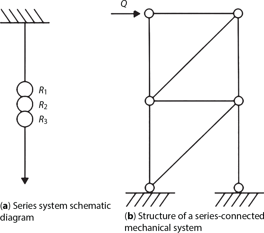
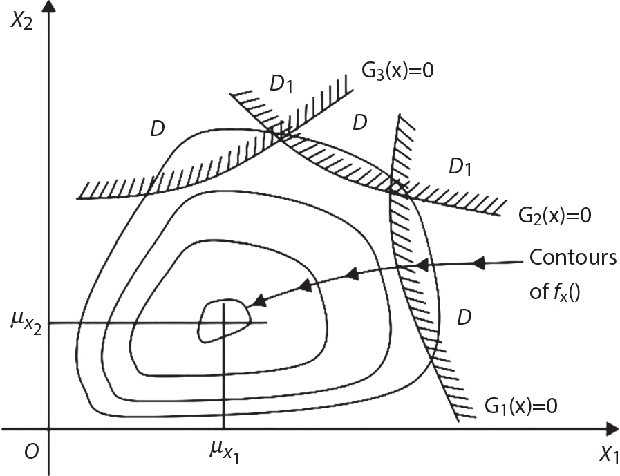
 . As can be seen in Figure 5.7, it is a complementary zone to the failure zone, marked as D and D1, and can be expressed by the following equation:
 is defined as the “validity of the ith mode” or Gi(X) ≥ 0. Thus, the validity probability is:
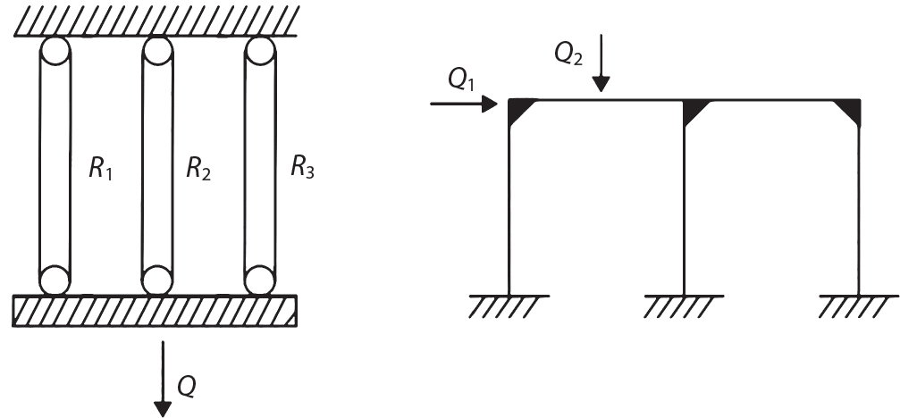
5.1.4 Practical Analysis of Structural System Failure

5.2 Calculation Methods for System Reliability
5.2.1 System Reliability Boundary
 represents structural failure occurring under the joint action of Mode 1 and Mode 2.
 :
:
 , as before, represents the probability of failure in that mode. The above equation can be expanded, achieving results consistent with that of Equation (5.18). In addition, as can be seen from Equation (5.18), if
  , then
  can be ignored, and Equation (5.20) can be approximated to Equation (5.21):
 , etc., in Equation (5.18). For the sake of description, it can be expressed as follows:
 . When
  is not considered, if
  is retained, then a lower boundary can be obtained from Equation (5.24) to ensure that each part exerts a non-negative effect [5-18] :
 and
and  can be alternated to combine all the terms containing k in Equation (5.24) to work out the maximum value of the lower boundary [5-19]:
 , and Pijk can be used to express
  , as follows:
 , then they will meet the equation below:
 .
.

 . Therefore, considering this change, boundary Equations (5.24) and (5.30) can be regarded as the boundaries of structural failure probability
  under sequential loads.
 of structural failure caused by the kth load under sequential loads. Equations (5.25) and (5.31) can also be used to work out the total failure probability under a complete sequence of loads, but at present, they are only interpreted as what exists under sequential loads.
 by estimation. One approach is to obtain a simplified solution by setting estimation undertow limit conditions: Fi, Fj are completely independent of each other or completely related to each other. If events Fi, Fj are completely independent of each other, Equation (5.32) can be simplified to Equation (5.20).
 , simplified as
  . This means that Equation (5.18) can be simplified to Equation (5.22). With both load sequence and multiple failure modes considered, the linear series boundary Equation (5.23) can be expanded, so
 represents the failure probability under the action of the jth load in the ith mode. For the terms on the right side, let
  :
:
 , which is obtained from
  is known, then
  . Thus, the cubic failure boundary can be transformed into the following formula, where Fi(i = 1, …, m) represents m possible failure probabilities [5-23]:
 ,
,  , where
  means that this part is not included unless it is positive.
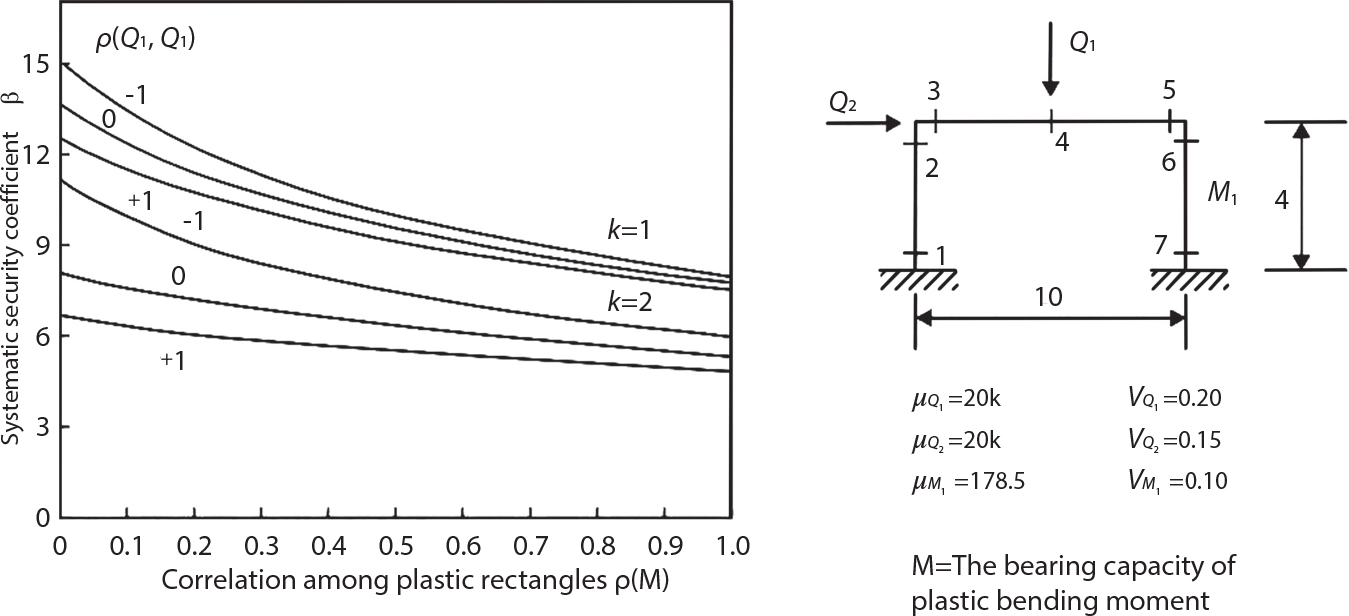
5.2.2 Implicit Limit State—Response Surface
 represent a series of points in X space, and then use the “responding surface method” to look for
  , an equation which is perfectly in line with the discrete value in
  . Normally, let
  be an n-order polynomial. The undetermined coefficients in this polynomial can be determined by minimizing the approximation error, especially in the zone around the design point.
 must be of equal order or lower in order than G(X). Higher-order
  will generate an ill-conditioned system of equations containing uncertain coefficients. It is also a non-steady-state equation.
 . However, quadratic polynomials are often used to estimate the response surface [5-29] [5-30] [5-31] [5-32] ;
 ,
,  are uncertain (regression) coefficients.
 , X = x, and the value estimated by Equation (5.42). This error is caused by inherent randomness and the “test for lack of fit” brought about using a simpler Equation, (5.42), to represent the actual limit state surface. It is impossible to separate them without performing an accurate calculation. However, an important step is to try to select regression coefficients A, B, C to minimize the total error.
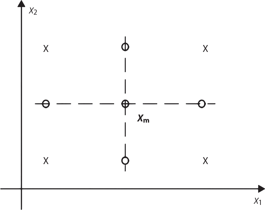
 in the experimental design, let Ei represent the value of the actual limit state equation, meaning the error represented by approximate surface Equation (5.42) will be
  . This can be done for each point in the experimental design. Now, the total error can be minimized. A very simple way is to use the least square fitting method, and use D to minimize the quadratic sum of errors
 i.e., an experimental design based on complete saturation, so that the surface should accurately coincide with the evaluation point £, especially with the mean point Xm, and point Xi = Xmi ± hiσi, where hi is any coefficient and σi is the standard deviation of Xi. According to these points Xm, an approximate surface
  can be accurately obtained at the postulated mean point. If the approximate surface falls in an optimal position, then the mean point Xm will coincide with the maximum likelihood point (design point), and the distance from the origin to these points will be the shortest in standard normal space.
 and named XD. These points are closer to the origin, so they are the best estimation points for the design point. When XD is known, the new mean point
  can be obtained by interpolation based on the linear relation between Xm and XD, as follows:
5.2.3 Complex Structural System
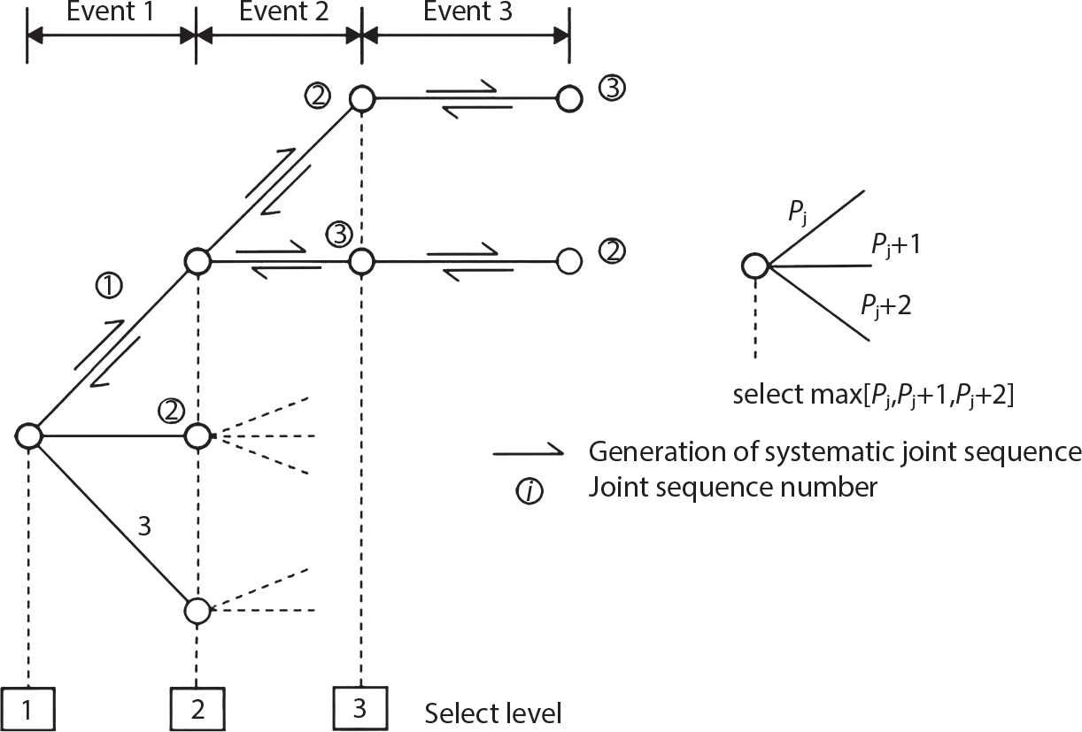
 :
:
 , so the use of Equation (5.47) is conservative, because fewer failure modes will be discarded. The mode failure probability calculated by Equation (5.46) may be bounded. For q ≤ n, the inequalities below are adopted:
 will be conservatively evaluated, and any mode that satisfies it will be ignored immediately.
 . The most important mode (the one that contributes the most to the estimation of system failure probability) is unlikely to be affected.
 is the vector of nodal force,
  can be called the “utilization matrix”, where Aij represents the number i of joints generated by pressure, because Q1 = 1 is the jth increment, such as the corresponding load increment rj. For a given failure model, given the joint sequence, Aij can be determined by traditional structural analysis. The inversion of Equation (5.53) generates an incremental effect rj, so that Equation (5.54) can be evaluated:
5.2.4 Physically-Based Synthesis Method
 , when it satisfies the Z function: Zext > [Z], the probability density of the representative point up is as follows
5.3 Example: Reliability of Offshore Fixed Platforms
5.3.1 Overview
5.3.2 Calculation Model and Single Pile Bearing Capacity

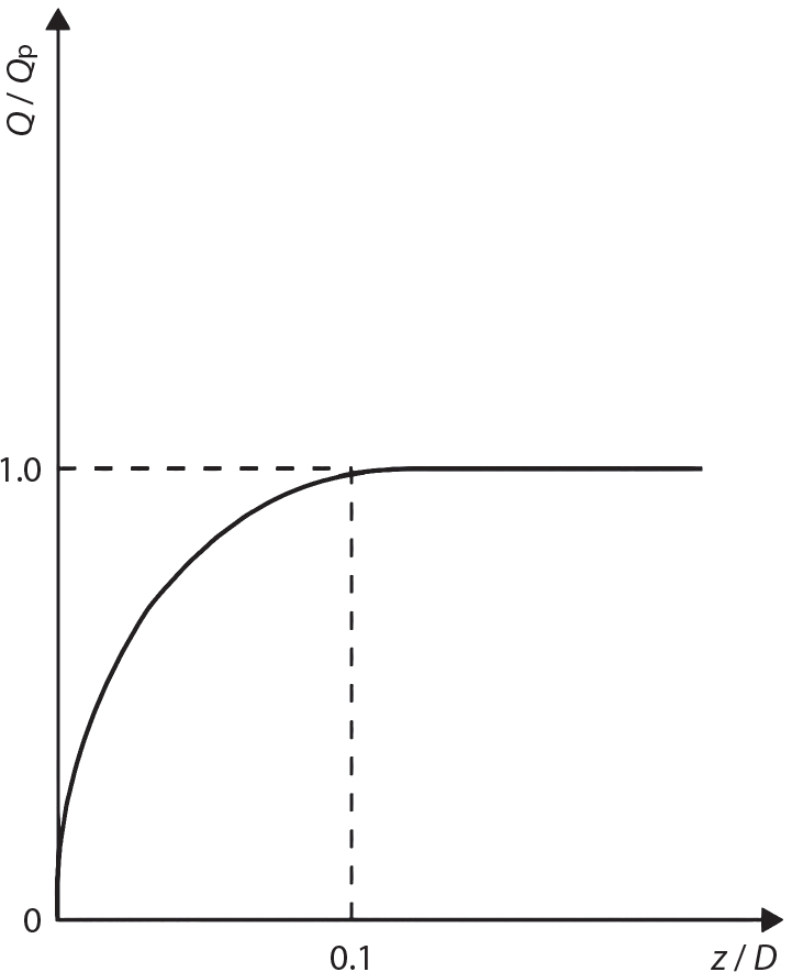
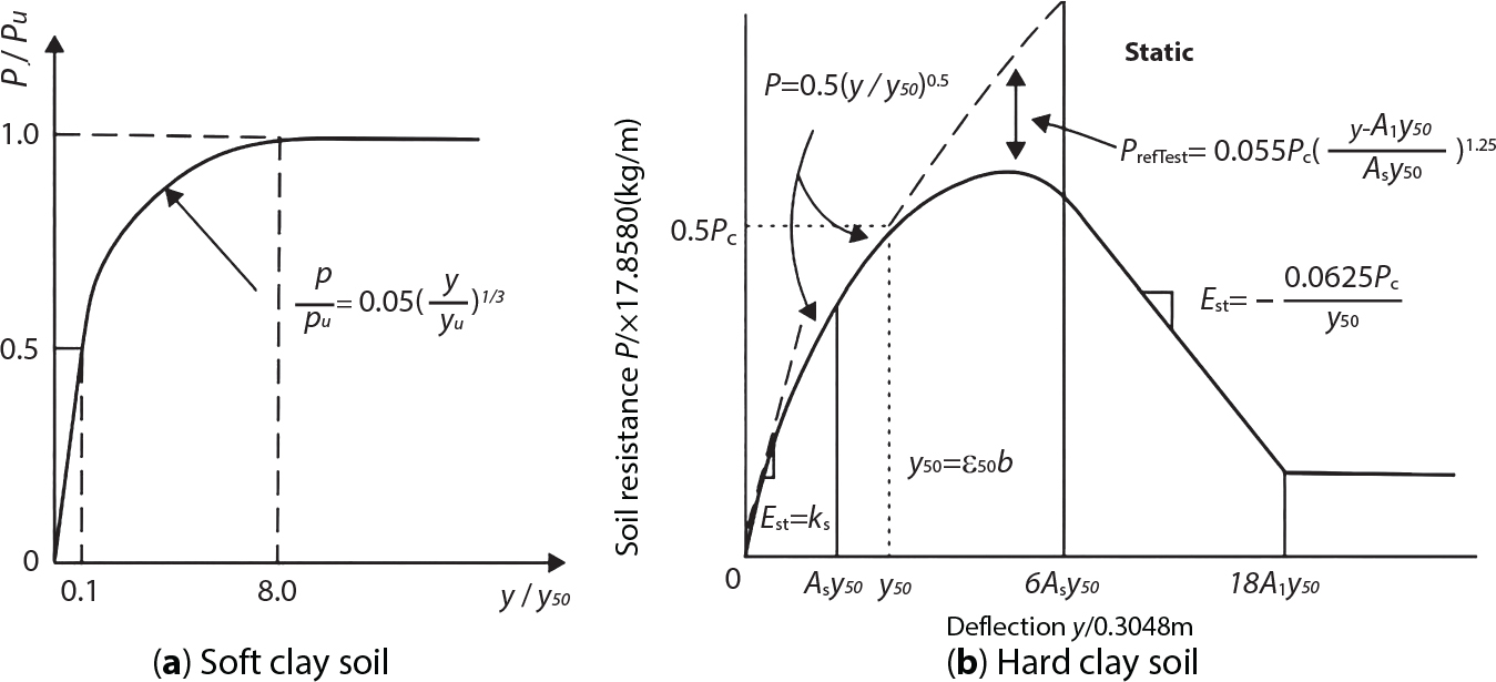
 is the empirical adjustment coefficient. K0 = 0.4 is the static earth pressure coefficient, Ka = tan2(45° − φ/2) is the Rankine active earth pressure coefficient,
  is the internal friction angle of sandy soil, β = 45° + φ/2, α = φ/2. The relationship between lateral load and deformation (p-y) of sandy soil can be calculated based on the following expression [5-56]:
5.3.3 Probability Analysis for the Bearing Capacity of a Single Pile
Depth (m)
Soil property
ϕ(o)
Su (kP)
r (kPa)
Limit side friction flim (kPa)
End supporting force qlim (kPa)
ε50(%)
k (MN/m3)
0.0 ∼ 2.0
Sand
33
109.0
15
1
5.5
2.0 ∼ 6.6
Sand
35
10.0
100
10
34.6
6.6 ∼ 7.7
Sand
35
9.0
40
1
5.5
7.7 ∼ 9.2
Clay
30
7.0
1.0
9.2 ∼ 30.4
Clay
75 ∼ 115
9.0
0.5
30.4 ∼ 48.5
Sand
34
10.0
120
12
34.6
48.5 ∼ 50.0
Clay
150
0.7
50.0 ∼ 69.3
Sand
34
10.0
120
15
34.6
69.3 ∼ 72.8
Clay
200
9.5
0.7
Soil parameter
Deviation
Cov
Distribution type
φ
1.00
0.15
Normal
Su
1.00
0.20
Lognormal
α
1.00
0.10
Lognormal
Nc
1.00
0.10
Normal
r
1.00
0.10
Normal
K
1.00
0.10
Lognormal
flim
1.00
0.15 ∼ 0.20
Normal
qlim
1.20
0.20
Normal
Nq
1.20
0.20
Normal
k
1.00
0.40
Lognormal
ε50
1.00
0.40
Lognormal
Computation model
Axial tension
Axial compression
Lateral displacement
End bearing
Soil property
Deviation
Cov
Deviation
Cov
Deviation
Cov
Deviation
Cov
Clay
1.00
0.15
1.00
0.15
1.00
0.30
−
−
Sand
1.00
0.15
1.10
0.15
1.00
0.30
1.20
0.15 
Load case
Deterministic analysis
Probability analysis
QD/Qmax
QD (MN)
Mean value (MN)
Coefficient of variation
Distortion
Steepness
Axial
Tension
39.6275
39.2930
0.1965
0.5355
3.0203
0.9916
Compress
130.3967
127.3500
0.1728
0.1558
3.1079
0.9766
Lateral
Δ = 0.5 m
54.1108
52.3160
0.0707
0.2234
2.8828
0.9668
Δ = 1.0 m
64.4857
62.3260
0.0642
0.3569
3.097
0.9665
Δ = 1.5 m
68.0915
65.559
0.0683
0.3345
2.9919
0.9628
Δ = 2.0 m
69.5433
66.7710
0.0699
0.2964
3.1358
0.9601 
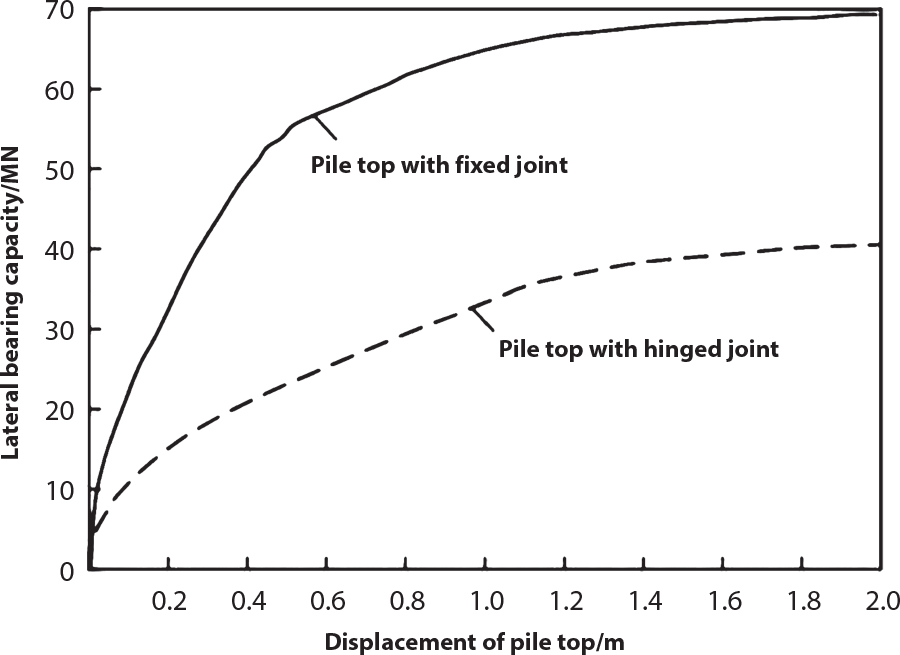
5.3.4 Bearing Capacity and Reliability of Offshore Platform Structural Systems
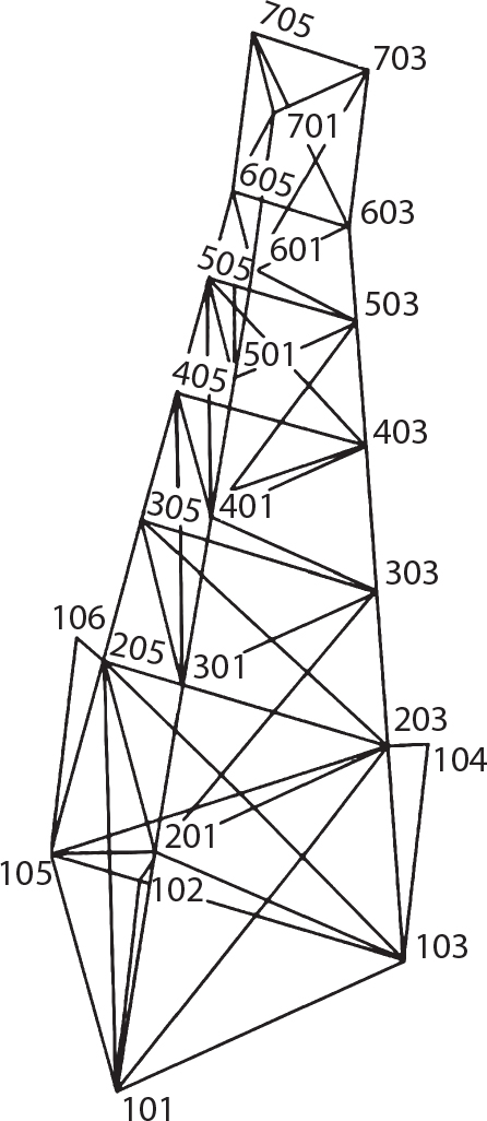
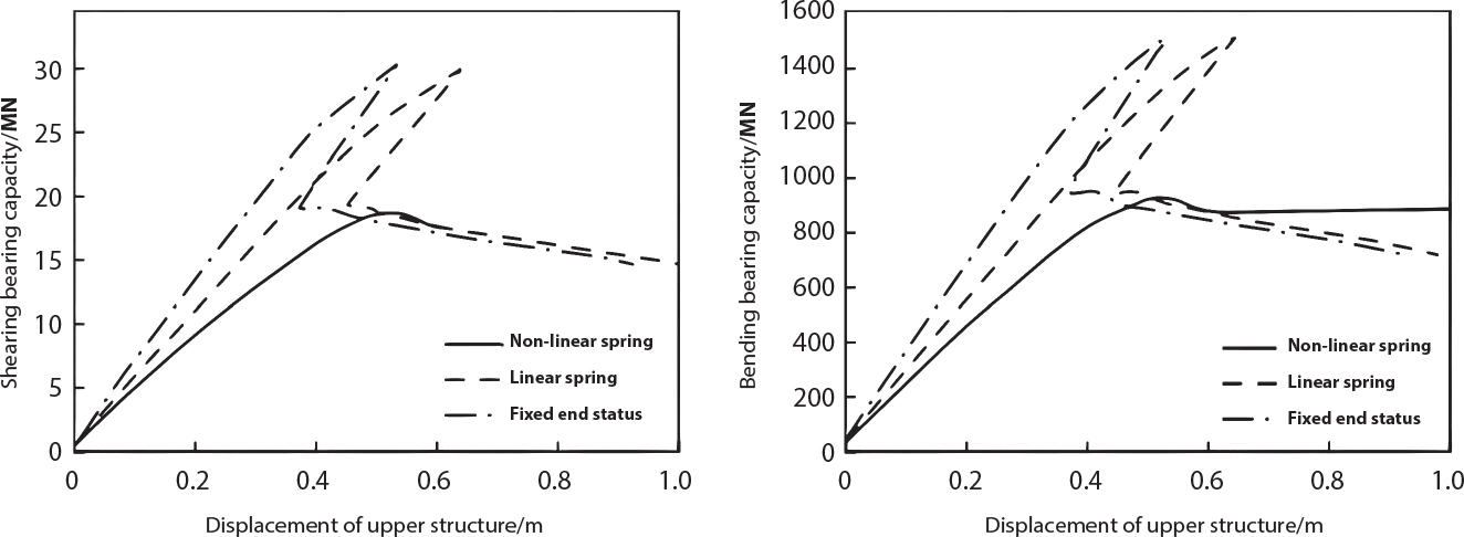
Load case
Fixed end at mud surface (MN)
Linear spring support (MN) on mud surface
Nonlinear spring support along pile length (MN)
1
30.3290
30.2160
18.8050
2
29.4800
28.4510
20.7260
3
30.4120
30.3600
18.3790
4
25.3900
24.6530
21.3690
5
26.0330
24.9970
21.7120
6
24.2760
23.7760
16.2270
7
27.4280
26.7620
17.8520
8
26.8507
26.5166
24.3330 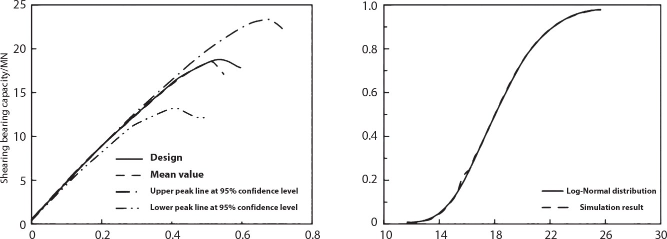
Load case
Base shear forceQ0/MN
QDeterm/MN
Average/MN
Simulation results
Qmean/QDeterm
Cov
Skewness
Steepness
1
4.7212
18.8050
18.3810
0.1468
0.4547
2.9568
0.9775
2
4.8076
20.7260
20.2020
0.1458
0.3471
2.6038
0.9747
3
4.3052
18.3790
17.9678
0.1469
0.4540
2.9526
0.9776
4
3.2770
21.3690
20.5430
0.1237
-0.1722
2.0835
0.9613
5
3.3761
21.7120
20.8200
0.1229
-0.1896
2.1231
0.9589
6
2.3665
16.2270
15.8360
0.1490
0.4471
2.9055
0.9759
7
2.9338
17.8520
17.4000
0.1484
0.4428
2.8899
0.9747
8
4.7057
24.3330
22.7930
0.0997
-0.5977
2.5059
0.9367
Average
0.1354
0.9672
Case
FORM
SORM
ISM-V
Pf
β
Pf
β
Pf
β
Cov
1
1.2219 (−5)
4.2199
1.1693 (−5)
4.2298
1.1619 (−5)
4.2313
0.0483
2
6.3284 (−6)
4.3660
6.0412 (−6)
4.3761
6.0098 (−6)
4.3772
0.0492
3
6.8924 (−6)
4.3473
6.5818 (−6)
4.3574
6.5466 (−6)
4.3585
0.0491
4
1.3328 (−7)
5.1457
1.2562 (−7)
5.1568
1.2553 (−7)
5.1569
0.0545
5
1.5367 (−7)
5.1189
1.4490 (−7)
5.1300
1.4478 (−7)
5.1301
0.0543
6
7.8598 (−8)
5.2439
7.3963 (−8)
5.2551
7.3957 (−8)
5.2551
0.0551
7
2.6681 (−7)
5.1038
2.5200 (−7)
5.0248
2.5163 (−7)
5.0251
0.0536
8
1.2663 (−6)
5.0138
2.5200 (−7)
5.0248
2.5163 (−6)
4.7168
0.0516
5.4 Analysis on the Reliability of a Semi-Submersible Platform System
5.4.1 Overview
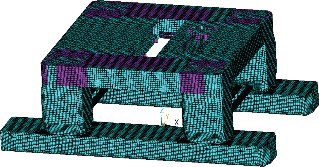
Working Conditions
Case Load parameters
1
2
3
4
5
6
7
Cycle (s)
9
7
8
9.6
7
6
9
Amplitude (m)
8.89
6.33
8.15
8.21
7.32
7.01
8.89
Incident angle (°)
90
120
135
180
180
90
180
Phase angle (°)
-33.6
160.2
108
133
40.1
-108
50
Working Condition
Sectional force
Fs (×107 N)
Mt (×108 N. m)
Fs (×107 N)
Mb (×108 N. m)
Fs (×107 N)
FTa (×107 N)
1
10.2
6.28
1.21
2.23
0.0025
2.92
2
2.66
24.3
1.38
3.76
0.24
0.0056
3
1.48
2.81
2.56
2.62
0.00075
0.0035
4
1.41
8.22
1.91
9.07
0.35
0.000031
5
1.57
5.79
0.7
2.87
6.43
0.060
6
4.06
4.06
0.014
4.13
0.00036
11.05
7
5.40
13.144
0.040
1.80
0.0030
0.0014
Parameters
Working Case
Still water
1
2
3
4
5
6
Wave amplitude/m
—
25
24
20
19
26
19
Amplitude extremum (×108)
3.42
2.84
75.4
0.74
16.4
2.30
3.00
5.4.2 Uncertainty Analysis
Variable
Distribution type
Variable coefficient
Average
Ru
Lognormal distribution
0.15
Calculation
Sw
Type 1 extremum
0.10
Calculation
Ssw
Normal distribution
0.02
Calculation
γu
Normal distribution
0.1
1
γw
Normal distribution
0.1
1
γm
Normal distribution
0.1
1
5.4.3 Evaluation of System Reliability
5.4.3.1 Analytical Process and Evaluation
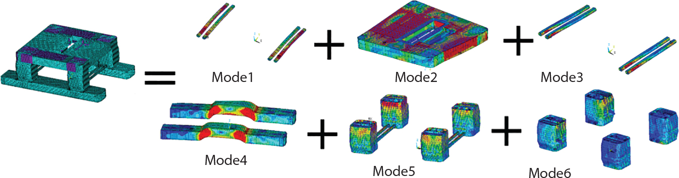

5.4.3.2 Reliability Calculation of Main Components
Variable
Distribution
Average
Standard deviation
Variance
Fu
Lognormal distribution
2.84×10⁸
4.26×10⁷
0.15
Fw
Type I extremum
1.02×10⁸
1.02×10⁷
0.1
γu
Normal distribution
1
0.1
0.1
γw
Normal distribution
1
0.1
0.1
γm
Normal distribution
1
0.1
0.1
Working conditions
Reliability index of various failure modes
Main structure (β & Pf)
a
b
c
d
e
f
1
4.00
8.77
6.66
7.28
12.91
7.88
4.00
3.16×10⁻⁵
2
8.44
4.38
6.23
5.56
110
9.89
4.38
5.93×10⁻⁶
3
9.39
9.59
4.11
6.73
12.96
10.00
4.11
2.01×10⁻⁵
4
9.43
7.98
5.13
2.38
11.43
9.85
2.38
8.70×10⁻³
5
9.35
8.98
8.38
6.46
4.87
9.98
4.87
5.58×10⁻⁷
6
9.24
9.95
10.00
5.24
12.87
3.23
3.23
6.18×10⁻⁴
7
6.18
6.47
20.32
7.87
12.89
10.00
6.16
3.6×10⁻¹⁰
5.4.3.3 Reliability Calculation for Local Nodes
Sectional force (×106N)
Working conditions
Distribution type
Variable coefficient
1
2
3
4
5
6
7
Lower buoy shear (×106N)
10.4
12.9
5.90
1.17
5.23
6.25
1.12
Type I extremum
0.10
Bending of cross brace end(×105N. m)
39.2
181
4.10
40.1
32.1
26.4
12.2
Type I extremum
0.10
Bending of lower column end(×107N)
37.5
6.20
3.44
54.8
35.9
34.3
4.83
Type I extremum
0.10
Shear of upper column end(×106N. m)
9.54
2.57
12.8
6.81
6.31
8.56
Type I extremum
0.10
Extreme value of sectional resistance
Average
Variable coefficient
Distribution type
Lower buoy shear (kN)
2.45×10⁷
0.15
Lognormal
Bending of cross brace end (kN*m)
3.35×10⁷
0.15
Lognormal
Bending of lower column end (kN*m)
1.12×10⁹
0.15
Lognormal
Shear of upper column end (kN)
2.27×10⁷
0.15
Lognormal
No.
Cases Working Condition
1
2
3
4
5
6
7
1
3.39
2.57
5.39
9.45
5.80
5.19
9.48
2
7.76
2.47
9.87
7.68
8.37
8.92
9.60
3
4.24
9.35
9.67
2.85
4.40
4.56
9.51
4
3.42
7.86
2.30
4.63
4.90
3.82
7.12
5.4.3.4 Calculation of Overall Platform Reliability
Parts
β & Pf
Cases
1
2
3
4
5
6
7
Main body
β
4
4.38
4.11
2.38
4.87
3.23
6.16
Pf
3.16×10⁻⁵
5.93×10⁻⁶
2.01×10⁻⁵
8.70×10⁻³
5.58×10⁻⁷
6.18×10⁻⁴
3.6×10⁻¹⁰
Node
β
3.21
2.26
2.30
2.85
4.381
3.81
7.12
Pf
6.64×10⁻⁴
1.19×10⁻²
1.07×10⁻²
2.19×10⁻³
5.91×10⁻⁶
6.95×10⁻⁵
5.40×10⁻¹³
Overall situation
β
3.20
2.26
2.30
2.29
4.36
3.20
6.16
Pf
6.87×10⁻⁴
1.19×10⁻²
1.07×10⁻²
1.10×10⁻²
6.50×10⁻⁶
6.87×10⁻⁴
3.6×10⁻¹⁰
References


