THE SPEED OF SOUND, the frequency of sound, and the wavelength of sound are fundamentally linked. By knowing two factors, it is possible to determine the third. The speed of sound is generally taken as a constant (c):
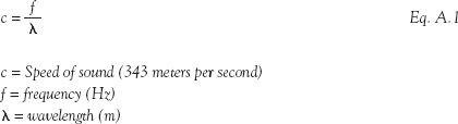
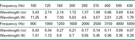
Table A.1 shows 1/3 octave bands with corresponding wavelengths.
Table A.1 Wavelength of sound waves at 1/3 octave bands given in meters and feet
THE LEVEL OF NOISE created by a source can either be expressed as a sound power level (SWL) or a sound pressure level (SPL). The term “SWL” is used for sound power levels because they are expressed in units of watts. The term “SPL” is used for sound pressure levels because they are expressed in units of Pascals. They both express the same thing: how much energy is used to create a sound wave.
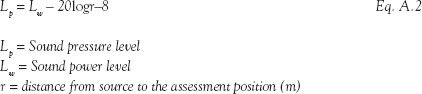
This equation assumes a point source in a hemispherical condition e.g., mechanical equipment fixed on a roof.
A.2.1 Adding sound levels
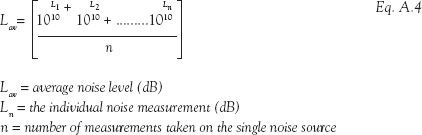
Because sound is measured on a logarithmic scale, adding together sound levels is not a linear process (i.e. 3 dB + 3 dB does not = 6 dB). To add together a number of sound sources in a room or outside a building, such as mechanical equipment, they must be logarithmically summed:
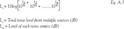
Once the difference between two noise levels is greater than 10 dB, there is no appreciable increase in the overall noise level. Table A.2 outlines how many dB should be added to a higher noise level dependent on the difference between the two noise levels.
Difference in dB between two sound levels | Level in dB to be added to the louder sound source |
0–1 | 3 |
2–3 | 2 |
4–9 | 1 |
10 or greater | 0 |
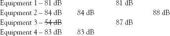
Table A.2 can be used as a simplistic method of adding noise levels, as shown in the example below:
Noise source 1 – 81 dB
Noise source 2 – 84 dB
Noise source 3 – 54 dB
Noise source 4 – 83 dB
Start by discounting any level which is –10 dB below any of the other sources (i.e., noise source 3). Next add the two loudest levels together (noise sources 2 and 4) using Table A.2. Then add the sum of these two levels to the remaining source (noise source 1).
A.2.2 Averaging sound levels
If you have several measurements of a single noise source taken over a number of separate surveys and find that the noise level varies, you may wish to average these noise levels. Because sound is measured on a decibel scale we cannot arithmetically average these levels and they must be logarithmically averaged.
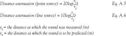
A.2.3 Sound propagation
For a point source (noise from a small single object), sound pressure will reduce at –6 dB for every doubling of distance. For a line source (such as a road or railway line), sound pressure will reduce at –3 dB for every doubling of distance. This is used to determine noise levels at a proposed building façade when the noise source has been measured at a position closer than the proposed façade.
A.2.4 Attenuation from barriers
The performance of an acoustic barrier can be determined by knowing the differences in the path length that a sound wave would have to travel to get over the barrier in relation to how far it would have to travel if the barrier were not there.
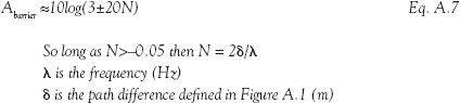
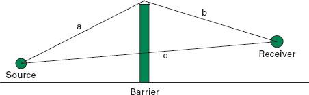
A.1 Attenuation of sound by a barrier

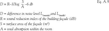
A.3.1 Noise break-in
The difference in noise levels from outside to inside a building can be predicted if the sound reduction or sound transmission index of a façade is known. The predicted level is dependent on understanding the level of absorption within the room:
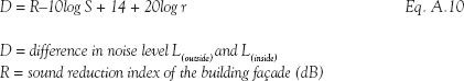
A.3.2 Noise break-out
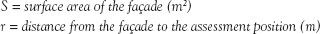
It is also possible to determine the level of noise breaking out from a room by knowing the properties of the façade and how far away the noise receiver position is:
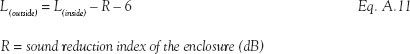
When constructing an enclosure around mechanical equipment, a more simplistic noise break-out calculation can be used to determine the insertion loss of an enclosure:
A.3.3 Sound transmission
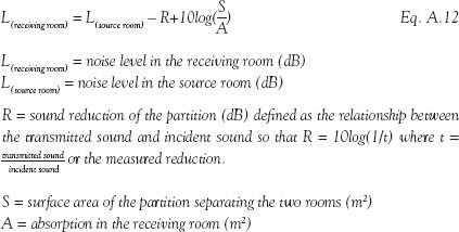
It is possible to predict the level of sound transmission from one room to another by knowing the insulation properties of the partition, the area of the receiving room, and the amount of acoustic absorption within the receiving room:
A.3.4 The resonance frequency of a single leaf partition
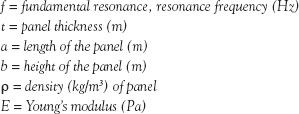
Where the stiffness of a partition is no longer the dominant factor in controlling sound transmission, a resonance dip will occur, resulting in a loss of performance. This is where the dimensions of a partition along with its material dictate its fundamental resonance, a frequency at which the panel will most easily vibrates. The resonance frequency of a panel can be defined from:

The density and Young’s modulus of some common materials are given in Table A.3.
A.3.5 The natural frequency of a twin leaf partition
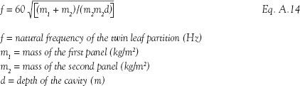
Just as it is possible to predict the resonance frequency of a single leaf partition, it is also possible to predict the natural frequency of a twin leaf partition. This can be defined as:
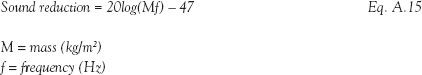
A.3.6 Mass law equation for separating partitions
The mass of a structure is the dominant factor in controlling sound transmission between the fundamental resonance frequency and coincidence frequency of a partition. The acoustic performance of a mass-controlled partition improves as the frequency of the sound acting upon it increases. It is therefore possible to make a simple determination of the level of acoustic insulation of a wall or floor for each frequency simply by knowing the mass of the structure.
Table A.3 Young’s modulus and density of materials
Material | Young’s modulus (Pa) | Density (kg/m3) |
Aluminum | 7 × 10¹⁰ | 2700 |
Brick | 1.6 × 10¹⁰ | 1900 |
Concrete | 2.4 × 10¹⁰ | 2300 |
Chipboard | 1.34 × 10⁹ | 695 |
Glass | 4 × 10¹⁰ | 2500 |
OSB | 3.5 × 10⁹ | 640 |
Plasterboard | 1.9 × 10⁹ | 750 |
Plywood | 4.3 × 10⁹ | 580 |
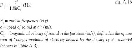
A.3.7 Critical frequency of a partition
The critical frequency limits the mass-controlled region and occurs where the wavelength of the incident-grazing sound wave is equal to the surface-bending wavelength of a material. The critical frequency can be calculated using the following equation:
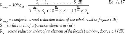
A.3.8 Composite partitions or façades levels
It is often the case that partitions are made up of several elements (e.g., a brick wall with a door in it or a concrete façade with a window). By knowing the sound reduction index of each element and its surface area, it is possible to determine composite insulation value of the partition:
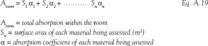
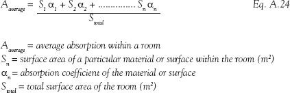
A.3.9 Absorption
The amount of acoustic absorption within a room is useful in calculating the total noise level within a space, as it quantifies how much sound is absorbed by things like surface finishes and even furniture. Appendix B details the absorption coefficient (a) of some common materials. By knowing the absorption coefficient of each surface in a room and its area, we can determine the absorption within a room:
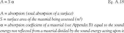
The total absorption within a room can be calculated by summing the area and absorption coefficients of each material or surface
A.3.10 Panel absorbers
For acoustically absorptive panels the mass of the panel, the distance the panel is set out from the wall or ceiling, and the frequency of the sound waves which cause it to sympathetically vibrate are linked (Figure A.2). By knowing two factors, it is possible to determine the third. This would allow you to determine how much space may be lost in a room as a result of having to set an acoustically absorptive panel a set distance from a wall in order to resolve a reverberation issue at a particular frequency.
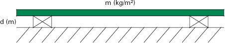
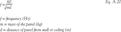
Table A.4 outlines cavity depths for panels with a mass of 2.5 kg, 5 kg, and 10 kg respectively, depending on frequency.
Panel absorbers are good at controlling reverberant sound at low frequencies partly because the cavity depths become impractically small above 250 Hz.
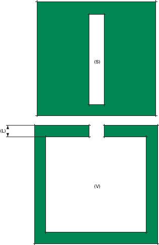
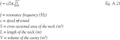
A.3.11 Cavity absorbers
Cavity absorbers, also known as Helmholtz resonators, are also intended for frequency-specific absorption. They are most useful at absorbing sound at the resonance frequency. This frequency is defined by the air volume inside the resonator as well as the dimensions of the opening (or neck). Figure A.3 and Eq. A.21 explain the relationship between these parameters and the resonance frequency.
Table A.4 Cavity depths in mm to achieve panel absorption for panels of three common weights
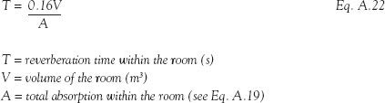
A.3.12 Reverberation time
Calculation of the reverberation is useful in determining how suitable a room is likely to be for its purpose. Table B.1 details optimum reverberation times for particular spaces, and this can be predicted prior to construction to ensure that a suitable environment will be designed using the following equations:
Sabine equation – more accurate for live rooms with small amounts of absorption and lots of reflections
Norris–Eyring equation – more accurate for dead rooms with high-level absorption and fewer reflections
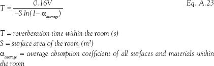
The average absorption of a room can be calculated by using the following equation:
A.3.13 Optimum reverberation times
These levels can also be predicted using the Stevens and Bates formula:
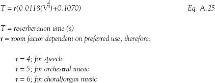
Note: This is the optimum reverberation time at 500 Hz. Add 30 percent to the result to determine optimum at 125 Hz. Reduce the result by 20 percent to determine the optimum at 4 kHz.
A.3.14 Speech clarity, C50
The equation to calculate C50 for a room, proposed by L. G. Marshall, is a weighted average of the values at the octave band frequencies between 500 Hz and 4 kHz, the range at which we find speech:

A.3.15 Music clarity, C80
The equation to calculate C80 for a room, proposed by L. Beranek, is an average of the values at the octave band frequencies between 500 Hz and 2 kHz:

Further reading
Hopkins, C. (2008) Sound insulation: Theory into practice. London: Routledge.
Sharland, I. (1972) Woods practical guide to noise control. Colchester, UK: Woods.