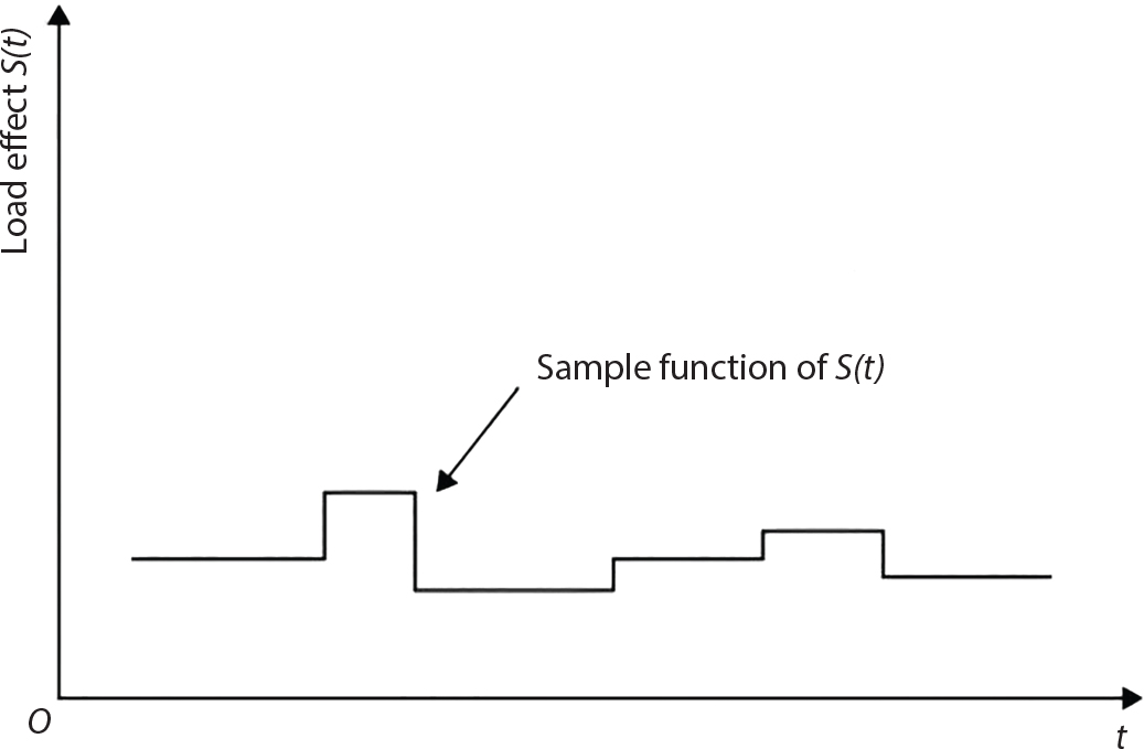
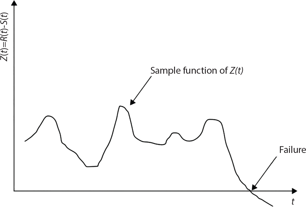
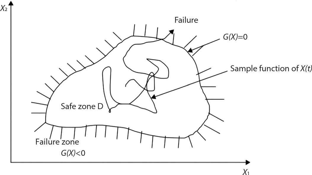
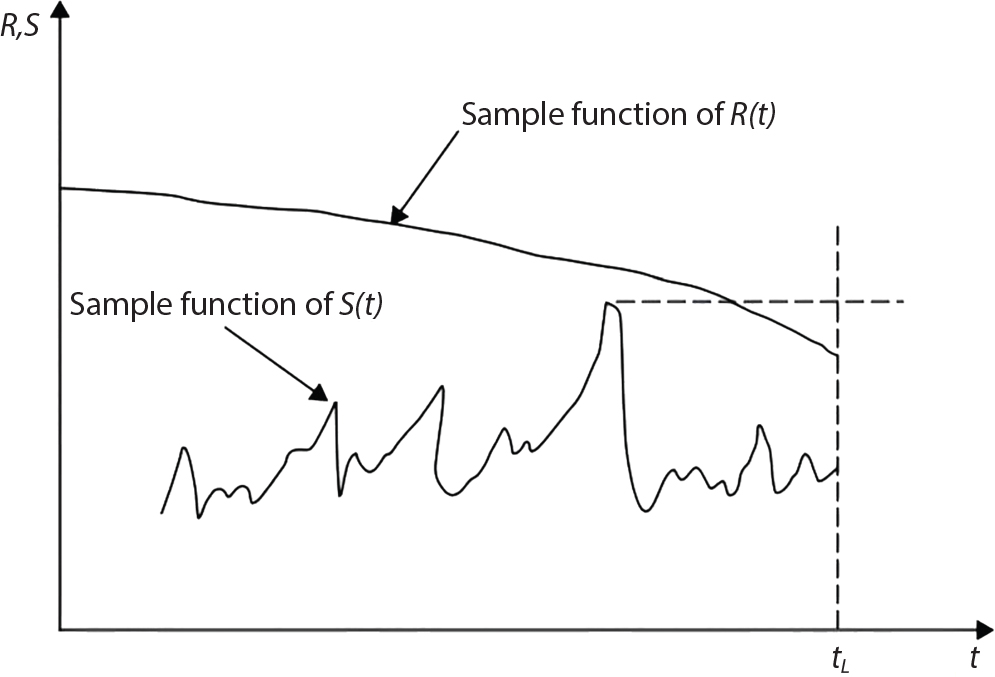
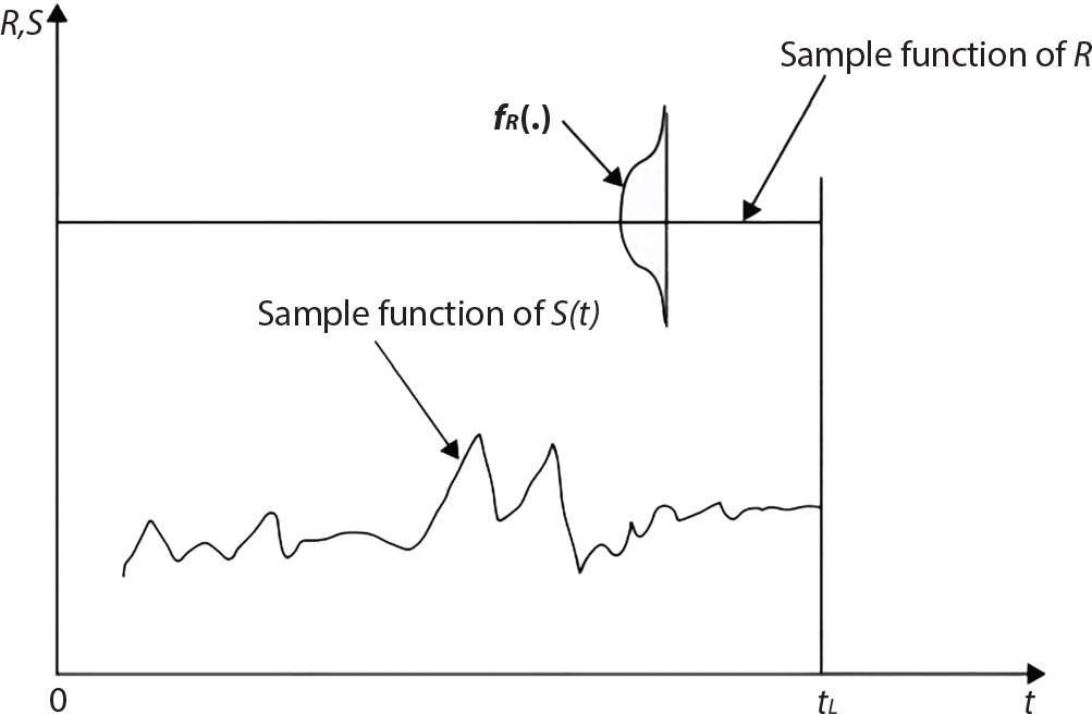
The external load borne by an engineering structure would change constantly, while structural resistance shows a time-dependent change trend, too. All this may cause a change in the reliability of the engineering structure. Usually, a basic random variable cluster may be defined as a function of time. As can be seen, whether the applied load changes with time (even for a quasi-static load, such as most floor loads) or the material strength changes with time (caused by load effect or corrosion), the structural response is bound also to change constantly with time. Fatigue and corrosion are two typical examples of structural strength degradation. The problem [6-1] of time-dependent structural reliability at a certain moment can therefore be expressed as Equation (6.1): where R(t) and S(t) represent time-dependent structural resistance and time-dependent load effect, respectively. If the transient probability density functions (PDF) fR(t) and fS(t) of R(t) and S(t) are both known, then the transient failure probability pf(t) can be worked out by convolution integral computation. Strictly speaking, Equation (6.1) makes sense only when the load effect increases suddenly at t or when the random load effect is reapplied at this moment. Otherwise, the structure will fail at an earlier time. The structure will not fail at a certain moment before t, i.e., it is assumed that the structure is always safe before t. Therefore, the load or load effect must change, and one of the following two situations needs to occur: So, Equation (6.1) can be expressed as For any given time t, the failure probability pf(t) can be expressed by the calculation method described in Chapter 3; X(t) in the equation is a vector composed of a set of random variables. Theoretically, the time interval [0, t] can be integrated by the transient failure probability expressed by Equations (6.2) and (6.1) to work out the failure probability of this interval. But in fact, the transient value of pf(t) is often related to the value of pf(t + δt), (δt → 0), since the random process X(t) is auto-correlative in terms of time. Figure 6.1 shows a typical sample function for the random process of load effect. The traditional processing method is to consider integrating the sample function presented in Figure 6.1, thus transforming it into a load or a load effect process, and expressing it in the form of extreme value distribution throughout the entire time interval. However, for this processing method, it is effectively considered that the structural resistance does not change with time. The improved method is to consider solving problems using the extreme value theory within a relatively short time interval (e.g., the duration of a windstorm or one year). This is like using the concept of a return period to calculate the failure probability of a structure in its service life. This method is very effective in calculating the failure probability of important structures such as offshore platforms and towers under discrete loads. Figure 6.1 Sample function of random process of load effect. Another way to calculate the failure probability of structures is to establish a limit state function (LSF) based on Equation (6.1): Then, we can calculate the probability that Z(t) will be less than or equal to zero within the service life of the structure. This is the so-called “crossing problem”. The moment at which Z(t) becomes lower than zero is known as the “moment of failure” in Figure 6.2, which is a random variable. The probability that Z(t) will become lower than zero within the service life of the structure is known as the “probability of first transcendence”. Figure 6.3 shows the situation in 2-D space. The “probability of first transcendence” refers to the probability that the random process vector X(t) will leave the “safe zone” G(X) > 0 within the service life of the structure. Because structural failure is defined as G(X) > 0, the “probability of first transcendence” is equal to the probability of structural failure. The concept of first transcendence is more universally applicable than the traditional calculation methods, and there is no formal restriction on the form of G(X). However, the knowledge related to random processes is required for calculating the first transcendence and accurately understanding its concept [6-2][6-3]. Figure 6.2 Sample function and failure time of safety limit state process Z(t). Figure 6.3 Transcendence of random process vector X(t). In the time integral method, the entire range [0, tL] of the service life of the structure is a unit, and the statistical characteristics of all random variables must be related to it. Therefore, the probability distribution of a load is the distribution of the maximum load within the service life of the structure. Similarly, the probability distribution of structural resistance is more concerned with the minimum value. But in general, the maximum load effect rarely occurs at the same time as the minimum resistance. Figure 6.4 shows the typical sample functions of R(t) and S(t). Figure 6.4 Sample function of nonstationary load effect and resistance. For most cases, structural resistance is time-independent, and in such circumstances, R(t) is a straight horizontal line, as shown in Figure 6.5. If R is a random variable, its actual value will be determined by PDF fR( ). In this case, Equation (6.1) may become where Sm(tL) refers to the maximum value of load effect within the service life of the structure, [0, tL]. The PDF of Sm( ) can be obtained directly by fitting previously observed extremum data with a proper PDF. The effectiveness of this method assumes that the statistical characteristics of load effect will not change in the future. Under normal circumstances, however, data will not always be valid for a long time, making it necessary to comprehensively analyze the extreme value distribution using updated data. Using the time integral method, we can apply a single-parameter load system Q to the structure at every other fixed time interval. In this case, the failure probability of the structure can be obtained by counting the number N of structural failures caused by the application of every independent load to the structure: Figure 6.5 Sample function of load effect and resistance (when resistance is constant). where n represents the number of times a certain load is applied; FN(n) is the cumulative distribution function (CDF) of N; LN(n) is defined as a “reliability function”. Because N is discrete, PDF fN(n) can be established as: Similarly, a “risk function” can be defined as follows: This function represents the probability that the structure will not fail under the first n − 1 loads, but will fail under the nth load. It can usually be expressed as a function of time. Suppose load application is time-independent, i.e., the ith time of application and the jth time of application are independent of each other. For the sake of convenience, we also suppose the PDF and CDF of resistance R and load effect S are known, and that both resistance R and load effect S (load system Q) are stationary random processes, i.e., PDF fR( ) and fS( ) are time-independent. Therefore, for the mutually independent loads applied to the structure, the probability that the maximum load effect will be less than a certain value can be expressed as: If n is very large, Equation (6.8) will gradually approach an extreme value distribution. If the failure probability of the structure can be expressed as after integration by parts, the following equation can be obtained Equation (6.10) expresses the extreme value distribution of the maximum load effect. Obviously, Equation (6.10) does not contain the number of times loads are applied, but is reflected in the distribution of S*. In engineering practice, many types of loads are often applied to the structure together. It is usually assumed that loads are independent of each another (e.g., live load and wind load), but in many cases this is not actually so (e.g., wave load and wind load). In addition, the peaks of different loads do not appear at the same time. Therefore, it appears very conservative to take the extreme value of each load. Usually, a loading process is selected to represent an equivalent load effect combination. The problem of load combination will be further discussed in Chapter 7. Essentially speaking, a problem of time-dependent reliability can be converted into a problem of time-independent reliability and then solved. First, it is necessary to investigate the maximum combination of various loads within the service life of the structure, and then calculate the probability that the limit state equation of the structure can no longer be satisfied under these loads. Equation (6.4) can be summarized as follows: where S( ) represents the load effect generated in the load process Q(t); R is a structural reactance vector defined in the PDF of structural reactance, fR( ). Because Equation (6.11) is difficult to solve directly, Wen and Chen[6-4] proposed using r in place of resistance R in Equation (6.11); the probability thus becomes a conditional failure probability pf(tL|r) and the failure probability can be expressed as where conditional failure probability pf(tL|r) is a function of a function of the random process of vector load Q(t). Importantly, it lists conditional failure probability under a given structural resistance. Now we can consider the problem to be the crossing problem mentioned above. Given the boundary of structural resistance R = r, we are concerned about the crossing probability of random load process Q(t). Suppose pf(tL|r) is related to the crossing rate. The previous crossing theory can now be directly used to calculate the failure probability. Because R and Q(t) are independent events, Equation (6.12) can be expressed as where Another similar way is to convert the problem of time-dependent reliability into a problem of time-independent reliability by means of an auxiliary random variable. It is first necessary to establish a limit state equation for time-independent reliability, and then to perform analog computation using FORM or the Monte-Carlo method. See Chapters 3 and 4. These methods have a shortcoming, however: conditional failure probability pf(tL|r) must be effective for all R and r, i.e., the replacement of the actual loading process with equivalent load effect is only effective within the linear elastic range (based on the principle of superposition) or ideal plastic range of the structure. Although the time integral method seems very simple to use, under the combined action of multiple loads, the random process theory is actually a better method for solving practical problems. When the discrete method is used to deal with the time-dependent reliability of a structure, the design reference period of the structure will be divided into several basic time intervals. These time intervals can be one year, or the duration of a special event, such as a windstorm. Thus, the problem of reliability is converted into a calculation of the failure probability of nL events that occur within a given time interval or within the service life of the structure. Once the service life of the structure, tL, is determined, the number of basic time intervals, nL, can also be determined. For a windstorm, although the frequency of its occurrence may be known, it is still impossible to accurately know its duration in advance. The discrete basic time interval could be one day, one month or one year, and it is most common to set it to one year. Thus, the calculation of failure probability discussed in the previous chapters is transformed into the problem of calculating the annual probability of failure. The resistance and load effect, variables people are concerned about, are transformed into the extreme value of the appropriate PDF for each year. The distribution of resistance and load effect needs to be determined according to observed data (e.g., the data on wind load and wave load), and the specific type of distribution depends on the length of the basic interval selected before. Therefore, the PDF of maximum annual wind force is different from that of maximum daily wind force, and these distributions can only be related to one another through some specific assumptions. The proof of the discrete method is analogous to that of the time integral method presented in the previous section, and can be divided into two cases: The structure may be subjected to various random loads at the same time. Given a time interval (e.g., one year), the value of nL can be very large, and the loads to be independent of one another. So, the extreme value distribution By Taylor series expansion where or The ignored second-order term in Equation (6.15) does not need to be included in the calculation unless the value of y makes Compared with the service life of the structure determined according to the number of loads, it is obviously more reasonable to take time as a parameter. The failure probability of the structure in time interval [0, t] can be expressed as where FT( ) is the CDF of time T, and LT( ) is the time-based expression of the reliability function. Let pi be the failure probability of the structure in the ith time interval, it can obtain Suppose pi is independent from time interval to time interval, pi = p and pt is sufficiently small. The failure probability can thus be approximated to It is similar to the results of Equation (6.17). Obviously, time can be determined arbitrarily. In most cases, the time interval is set to one year. The failure probability of the structure within the service life [0, tL] can be written as The failure probability pi of the structure in the ith time interval depends on the number of loads applied during this time interval. If a basic time interval is regarded as an event, such as a windstorm, then the actual number of loads in this event can be ignored, and an approximate extreme value probability distribution is used to describe the maximum load effect In order to obtain the failure probability pf(tL) of the structure within its service life, the frequency of event occurrence needs to be given in advance. Suppose the probability that k events will occur in the time interval [0, t] is pk(t), then the failure probability of the structure in the time interval [0, t], like Equation (6.14), can be expressed in time a: where all possible frequencies of the occurrence of the event are considered. Suppose pk(t) obeys the Poisson distribution: where ν represents the average rate at which events occur. According to the characteristics of the Poisson distribution, this means that the e specimens are independent of one another and do not overlap. This assumption will be quite reasonable when ν is small enough. By substituting Equation (6.23) into Equation (6.22), we get: where It must be noted that some external information needs to be taken into consideration for the calculation of the failure probability Suppose Hk > 0 in the equation, then the PDF The return period refers to an average time interval within which an event that exceeds a certain level or load recurs within a certain statistical period. According to this concept, the return period can be regarded as the reciprocal of failure probability in the limit state. So, in a broad sense, the calculation of the return period can be defined by the following formula: where Taking this idea further, if there are m mutually independent random loads affecting the failure probability, then: or This equation shows that the reciprocals of the return period can be added together, provided that the events in each basic time interval are independent of each another. Another f analysis index frequently used in classical reliability theory is the “risk function”. This can be expressed either by the number of loads applied or by time. As can be seen from Equation (6.18), the structural lifetime expressed with time as a parameter is P(T < t) = FT(t), and the PDF of the designed service life is: This is also called “unconditional failure rate”, because it reflects the failure probability between time interval t and t + dt when dt → 0. The risk function (also known as the “year-specific failure rate” or “conditional failure rate”) expresses the failure probability between time interval t and t + dt when dt → 0. Furthermore, it is assumed that there is no failure occurring before t. So or This equation shows that, when FT(t) is very small, hT(t) is very close to fT(t). Figure 6.6 shows some typical risk functions. By substituting Equations (6.18) and (6.20), we can transform Equation (6.33) into: and where the integral term in the brackets represents total failure probability. Therefore, if any of fT(t), FT(t) and hT(t) is known, the remaining two can be obtained by calculation. For a typical structure, the risk function is usually a “bath-tub” curve (see Figure 6.7). The figure shows that the risk is highest at the initial stage, and reduces rapidly with the gradual application of load. This stage is mainly a period during which a test load is applied. As time goes by, the structure gradually deteriorates, while risk rate increases. Figure 6.6 Typical risk function. Figure 6.7 Variation trend of risk function in different structural stage. In the time-dependent reliability method, the failure probability of the structure can be directly estimated by calculating the probability of first transcendence. For a highly reliable system, this is a feasible approach. If the random process S(t) has a safe zone DS within the service life of the structure, [0, tL], then the structural reliability can be expressed as: where [0, tL] represents the service life of the structure or other time intervals concerned; R(t) represents the structural resistance at t; S(t) is also the random process of load effect with time as the independent variable. For the sake of operation, it can be expressed by the formula below: Usually, there is no simple corresponding relationship. At present, for the most commonly used method, based on the random process theory, a upper bound relation between the failure probability and crossing rate is put forward as follows: where pf (0) represents the failure probability of the structure at t = 0 or at the exact moment when load is applied. The results are valid for the random process of a stationary vector load. If the random process of the vector load is smooth, the term Obviously, there is an error in the calculation formula because the reference source is not found! Three problems need to be paid attention to. The first involves calculating the term pf (0), which is a non-time-dependent probability and can be calculated directly by any of the methods presented in Chapter 3. The second problem involves calculating the crossing rate. The method discussed in Section 6.5 can be used. After these conditional terms are obtained, the integral term in Equation (6.12) is needed to calculate the unconditional failure probability. The third problem concerns the degree of closeness between the upper boundary in Equation (6.37) and the real results. For the random process of a narrow-band load, crossing phenomena are rather concentrated, and in this case, the upper boundary expression will be overestimated; conversely, if the random load vector is not a narrow-band random process, then the upper boundary estimation will be quite accurate. Another way to evaluate the time-dependent reliability is to bypass the calculation of the crossing rate and evaluate the probability of the random m-vector process in the given failure domain by simulating the random process of every continuous vector [6-6]. In particular, the random process of every standard multivariate Gaussian can be represented by the trigonometric series of random coefficients [6-7]. Then, by using directional simulation, the probability for the random process to cross the security domain is calculated by maximizing the service life of each directional sample. Although this method is straightforward, it still has a disadvantage, i.e., a heavy calculation burden, because it needs at least s(t +1) simulation runs; s represents the number of components of the random vector process and t represents the number of parameters used to express the random process. An optimal value for t has not yet been determined, but it may be quite important. This method for evaluating the time-dependent failure probability is often used to check the results obtained by other methods [6-8]. The integral of Equation (6.12) may hardly obtain an exact analytical solution. The same problem exists in Equation (6.37). The trick is to use numerical simulation, FORM, etc., to solve these. (1) Importance sampling and conditional expectation sampling Importance sampling is adopted for Equation (6.40) while conditional expectation sampling is adopted for Equation (6.39) [6-9]. Importance sampling is expressed as follows: The failure domain D is first integrated. The limit state equation is G(x) = 0. m independent limit state equations constitute The term { } in Equation (6.39) is replaced with As can be seen, Equation (6.40) is of the same form as the time-dependent reliability function Equation (6.12). The m-integral on D1 can be obtained by Monte-Carlo simulation based on importance sampling PDF hv( ). If the term { } in Equation (6.39) can be calculated numerically, then every sample in the importance sampling method can be calculated as well. In this way, the conditional expectation gap can be narrowed, thereby reducing the number of Monte-Carlo samples required. When the directional simulation in the load random process space is closely related to obstacle crossing, as shown in Figure 6.8, then the random process space will be the load random process Q(t). In load random process space, the security domain SD can be interpreted as structural resistance, denoted as R = r. The traditional limit state equation Gi(q, x) = 0, i = 1, …, k can be interpreted as the boundary. Let the joint PDF of resistance R be fR( ), and be the function of other random variables, R= R(X). The components of X can be structural components or the components of resistance, material properties, etc. (X contain the uncertainties arising from load random processes. Q(t) can contain stochastic processes other than load random processes. Its PDF must reflect the independence of load components.) Figure 6.8 Sample functions of vector stochastic processes. Structural failure probability can be provided in Equation (6.12). Given the structural resistance R = r and the conditional failure probability pf(tL | r) of the highly reliable structural system in the time interval tL, a calculation can be made by means of Equation (6.24) or (6.38) according to the crossing rate where pf(0,s | a) is the failure probability at t = 0, and where A is the directional cosine vector, fA( ) is the PDF, S is the radial distance representing structural resistance, and fS|A(s | a) is the conditional PDF. For a given limit state equation, Gi[X(t)]≥0,i = 1,…,n, the security domain DS can be obtained. Moreover, pf(0) and The main problem that remains is how to calculate the integral of the resistance R, which is a random variable. An important way presented in Section 6.2 is to introduce an auxiliary random variable to transform the problem of time-dependent reliability into one of time-independent reliability. However, experience shows that, if the limit state equation is time-dependent, or if the random process is non-stationary when an auxiliary random variable is adopted for calculation, then the calculation will take much more time [6-10]. In addition, the Laplace integral method can be used for calculation [6-11]. The traditional first-order second-moment method is highly effective in analyzing problems of time-independent reliability, but ineffective in calculating the crossing rate with respect to the problems of time-dependent reliability. The main reason for this is that there must be structural resistance R, which must be a time-independent random variable during the process of integration. For this reason, the importance sampling method and Monte-Carlo simulation have become the most practical methods. It is very important to perform a dynamic structural analysis when the structure bears a time-dependent load which affects the structure’s response to the load (e.g., deformation and stress). In traditional structural dynamic analysis methods based on time-domain analysis, the structural dynamic equations are integrated over time. The load changes over time, and structural response is also a function of time. This whole calculation process can be accurately applied to a very complex structure. Material and structural properties can also be nonlinear, but iteration is required during calculation and is highly time-consuming. If the load is stochastic, then the time-domain-based calculation results will have limitations since the load can no longer be described based on time. A common practice is to analyze structural response by a sample function of load, and then to observe the statistical characteristics of the response by constant repetition. If there is a maximum allowable stress and deformation set under the design standards, then the limit state equation G(x) = 0 can be established. Therefore, theoretically at least, the structural reliability can also be calculated by the Monte-Carlo method. Unfortunately, this method is not so practical in practice, because it requires a lot of time-domain-based analyses, and each analysis is highly time-consuming. Therefore, it is quite difficult to combine traditional dynamic analysis with structural reliability problems unless the random process theory can be further simplified. For this reason, the time domain method remains poorly applicable to the theory and application of structural reliability. When the structure is linear, i.e., when it is an elastic structure based on the assumption of infinitesimal deformation, or when the input-output (e.g., load-stress) transformation equation is linear, a calculation method based on the frequency domain can be used. This method is widely used to solve random vibration problems [6-12]. A stationary random process X(t) can be decomposed into a finite number of sine and cosine components, each of which has its stochastic amplitude and natural frequency. This is the famous Fourier integral transform. The coefficients of cosine terms are determined by the integral of the production of the random process X(t) and cosωt. The same is true for the coefficients of sine terms. Every term is a Fourier transform of X(t). Because the randomness of X(t) is determined by the autocorrelation function RXX(τ), the Fourier transform of X(t) can also be expressed as a function of RXX(τ). The coefficients of the cosine terms can be expressed as a continuous function of ω: Because RXX(τ) is a symmetric function, the coefficients of the sine terms corresponding to Equation (6.43) are zero; of course, SX(ω) is also a symmetric function (see Figure 6.9 (a)). SX(ω) is what we usually call the (mean squared) spectral density. It is not hard to see that, if X(t) is completely disordered, RXX(τ) obtained from Equation (6.43) will be zero (except where τ = 0), and SX(ω) is a constant for all ω. This is what is known as white noise. Due to the lack of prominent frequency components, its power is the same across all frequency bands (see Figure 6.9 (b)). Similarly, if there is a dominant frequency near ω0 for the random process, then the form of the spectral density is shown in Figure 6.9 (c)). This is the narrow-band process, which is of great importance for structural dynamic analysis because most structures have a major vibration mode or response frequency. This mode usually corresponds to the (minimum) natural frequency of structures. Let τ in Equation (6.43) be zero, and integrate both sides in (−∞, ∞), so The area enclosed by the curve SX(ω) is the mean square value of the stationary random process X(t), equivalent to its variance (see Figure 6.9 (a)). Let uX = 0, since randomness is the main concern here. The analytical results for uX ≠ 0 can be directly superimposed on the stochastic results at ux = 0. In addition to the variability of random processes, the probability distribution of peaks is also a key concern. It is denoted as Fp(a), i.e., the probability that the peak of random process X(t) lies below the horizontal line X(t) = a, when uX = 0. The results achieved in the previous section can be used directly here. For a narrow-band random process that is smooth enough, it will have a maximum at X = 0 only. The ratio of X > a is Figure 6.9 Sample function and spectral density of random process. Figure 6.10 Probability density function of Rayleigh distribution. For the horizontal line x = a, the following is obtained after differentiation: Equation (6.49) represents a Rayleigh distribution (Figure 6.10). Obviously, fp(a) reaches its maximum at a = σX. There is no peak at a = 0. If the random process is not completely smooth, e.g., if there are multiple extreme values every time it transcends zero, or if the random process X(t) does not obey normal distribution, it is more appropriate to describe the probability distribution of the peaks of the random process by the more generalized extreme value distribution (e.g., EV-III). It should be noted that the spectral density of structural deflection or stress at a certain point can be obtained by considering the excitation-response relationship of the linear structure in the frequency domain, and the corresponding relationship will be as follows: Figure 6.11 Analysis on the relationship between input and output spectral density function of offshore platform structure. For a single input source or a load random process X(t), a single output Y(t) can be generated. H(ω) is a frequency-response function. Equation (6.50) can be generalized as a linear superposition of multiple independent inputs: When there is a correlation between inputs, there will be a more complex relationship between input and response. Figure 6.11 shows the main principle by which the frequency-response function is used to obtain the output spectral density from input spectral information. The input spectral information can be inferred by observation and physical process analysis. H(ω) can be obtained based on the system analyzed or by integrating the structural response in a given excitation mode A very important problem related to time-dependent reliability is fatigue. This is also a typical limit state, i.e., it is controlled by the number and intensity of imposed loads rather than by a single load. The limit state equation of fatigue can be described as: where Xa represents the actual structural strength or performance. Xr represents the structural performance that must be satisfied within the designed service life. Therefore, if the fatigue life is expressed by the number of stress cycles, Xa becomes the number of stress cycles needed to cause structural failure and Xr becomes the number of stress cycles that can still meet the design requirements within the given service life. Correspondingly, there are some cases in which the fatigue life is described by means of crack size, damage index, etc. In general, both Xa and Xr are uncertain, and their accuracy depends on the fatigue model adopted. The equation below provides a traditional model that can be used to describe the fatigue life Ni of a component or structure under constant stress: where K and m are usually constants, but here, they are random variables; Ni represents the number of stress cycles at constant stress amplitude Si. The value of K and m can be evaluated by experimentation. In general, a conservative value is adopted in Equation (6.53) to ensure that the fatigue life Ni can be assessed safely. For structural reliability analysis, Equation (6.53) needs to be closer to reality rather than being a conservative prediction. Therefore, the value of K and m presented in the reference literature may not be applicable in practice. In addition to the applicable expected value, it is also necessary to consider the impact of the uncertainty of these parameters. As for the analysis method, please refer to traditional structural reliability analysis. For the safe domain, Equation (6.52) can be rewritten as: where N0 represents the number of cycles that the structure must be able to bear in order to meet the design requirements; N0 also contains uncertainties. In engineering practice, the stress amplitude is not a constant, but a random variable. If the amplitude in each cycle can be recorded, then the linear damage accumulation rule can be applied: where ni represents the actual number of cycles under the action of stress amplitude Si; Ni represents the fatigue life under the action of stress amplitude Si. If stress amplitude varies, Equation (6.55) is turned into: where N represents the total number of amplitude cycles. Traditionally, the damage parameter Δ is a uniform value, but in fact, it ranges from 0.9 to 1.5. Therefore, Δ reflects the fact that great uncertainty is caused in practical application due to the empirical problem of Equation (6.56). It is roughly reasonable to adopt a lognormal distribution with a mean of 1.0 and a coefficient of variation of 0.4∼0.7 [6-12][6-13]. When equation (6.56) is used, it is necessary to determine the N value and the probability distribution of Si. There are many different methods for extracting the N value. The safety domain can be redefined with damage parameters: where X0 is used to solve the uncertainty problem caused by failure to accurately determine stress amplitude Si during the application of Equation (6.53) in the model. The main difficulty encountered in applying Equation (6.57) is that the N value is uncertain. One way is to divide the stress amplitude into l groups (where l is a given number), and the number of cycles in each group, Ni, is uncertain, so Another way of using the fatigue model is to consider crack propagation under the action of cyclic or random load, but this method is not always effective [6-14][6-15]. The experimental results show that the crack propagation rate da / dN depends on the change amplitude Δk of the stress intensity factor: where a represents the current crack length; N represents the number of stress cycles; C and m are testing constants, usually dependent on the frequency of load application, the average load and the testing environment. During reliability analysis, C and m must be processed as uncertainties. Generally speaking, the stress intensity factor does not change significantly with stress, so the change amplitude of the stress intensity factor can be calculated by: where ΔS represents the applied stress amplitude; K(a) is a function of the current crack length a; ΔKth is the threshold of ΔK, and ΔK = 0 at ΔKth. After N stress cycles, the variability of the current crack length a can be obtained by integrating Equations (6.59) and (6.60): where a0 represents the initial crack length. After obtaining the statistical characteristics of the parameters in the equation, we can obtain the mean and variance of a(N). The variable-amplitude load ΔS depends on the load sequence, and is a random variable. This problem can be solved by the incremental method according to Equation (6.60) or by using an effective ΔK [6-14]. For either method, the limit state Equation (6.52) can be rewritten as: where aa represents the limitation of the crack length under certain functional conditions after the structure has borne N load cycles within the designed service life tL. Another method for the limit state equation is to express it by means of the crack tip displacement, which represents the material stiffness [6-14]. (1) Probability model of fatigue load Under the long-term action of random loads such as wind, waves and currents, marine structures will produce alternating stress, micro-cracks and continue to expand, resulting in fatigue failure of these structures. Existing engineering experience shows that once the fatigue problem of an offshore structure occurs, it will lead to serious consequences. Before carrying out fatigue life analysis of a platform structure, it is therefore necessary to understand the fatigue load of the structure first. The mooring force and motion parameters of a BZ28-1 SPM (Single Point Mooring) system are derived from the model test conducted on the Dutch ship model test pool in 1986. By analyzing the test data [6-16], the nonlinear relationship between mooring force and wave environment parameters can be obtained, which is convenient for the fatigue life analysis of a jacket structure. ① Statistical characteristics of environmental loads Because the symmetry of the platform structure and the statistical characteristics of the ocean state in each direction are quite similar, 11 ocean states in the three wave directions of 0°, 45° and 90° (corresponding to the east, northeast and north, see Figure 6.12) are considered for fatigue calculation and analysis. Each direction has the same probability of occurrence P, and it is assumed that the probability of occurrence of waves and current in the same direction and wave and currents perpendicular to each other in these three wave directions account for half of each other, as is shown in Table 6.1 and Table 6.2. Figure 6.12 Coordinate system of a single point mooring offshore jacket platform. Table 6.1 Statistical standard deviation of high frequency mooring force range. Table 6.2 Statistical standard deviation of low frequency mooring force range. ② Distribution of environmental load The distribution of load during the whole lifetime of a structure is usually referred to as the long-term distribution of fatigue load, but the fatigue life of a structure is normally unknown when fatigue life analysis is carried out. Therefore, the representative distribution of fatigue load over a certain appropriate time length is usually regarded as the long-term distribution, which is known as the recovery period of a load spectrum. The long-term distribution of the load spectrum is composed of a number of short-term ocean conditions, while the distribution of wave height and mooring force of each short-term condition is assumed to be a Rayleigh distribution, which can be expressed as: Where P (H) is the probability density function of the corresponding wave height. This means that the number of cycles between the wave height H and H +ΔH is where: n is the number of cycles of ocean conditions during the recovery period. According to the Rayleigh distribution, every effective wave height Hs can be discretized into a series of regular waves with wave height Hd. The discrete wave train contains the maximum wave height that may occur within 100a. After discretization, the corresponding number of cycles of wave height in a 1a recovery period is shown in Table 6.3. Following the Rayleigh distribution and if the mooring force and wave height have the same probability density function, the discrete mooring force sequence will be as shown in Table 6.3. In this way, the high- and low-frequency mooring forces corresponding to each discrete wave train can be obtained, where Fu and Fz are the horizontal and vertical discrete mooring force sequences, respectively. The number of cycles of the discretized high-frequency mooring force in 1a recovery periods is the same as that of the waves, as shown in Table 6.4. The number of cycles of low-frequency discrete mooring force sequences in 1a recovery periods is shown in Table 6.5. (2) Fatigue life assessment ① Numerical simulation of a platform structure The substructure method is used to analyze the pile-soil interaction of an offshore jacket platform, which involves the total structure being subdivided into upper jacket structure, pile, and foundation soil subsystems at the pile head. After this, the single reaction is combined to satisfy the interaction conditions, after which the reaction of the whole structure can be obtained. Table 6.3 Mooring force discovery series under different effective wave heights. The Winkler foundation beam model is used to simulate the dynamic interaction between pile and soil. The soil is treated as a Winkler foundation, and the pile consists of a long beam buried in the soil. When analyzing the bearing capacity of a single pile, the finite element model is used to carry out the calculation. The construction can be seen in Chapter 5. The deterministic analysis method (also known as the discrete wave method) is used to analyze the effects of wave and mooring loads on the platform jacket structure. Generally speaking, this includes the calculation and analysis described hereafter. The quasi-static analysis of the structure can be carried out under different ocean conditions. Depending on the fatigue load condition determined at the front, linear wave theory can be applied to calculate the wave force acting on the conduit frame according to each wave height and period for the wave condition. For the mooring force, the discrete horizontal and vertical mooring force components are directly applied to the top of the column, after which the internal forces and stresses on the members can be obtained by finite element analysis of the platform jacket structure. Considering the stress concentration of the corresponding welded tubular joints in the structure, the hot spot stress range of the tubular joints can be obtained by multiplying the calculated nominal stress by the corresponding stress concentration factor, which can then be used for fatigue life analysis. Table 6.4 Wave ocean state distribution. ② Cumulative fatigue damage and life assessment method The long-term distribution of stress range is composed of a series of shortterm Rayleigh ocean conditions. The fatigue loads of the single-point mooring jacket platform structure include wave forces, high-frequency mooring forces and low-frequency mooring forces. The fatigue life of a BZ28-1 SPM jacket structure has been analyzed by the China Classification Society [6-17], where the fatigue damage caused by these three forces is calculated separately. After this, the total damage can be obtained by adding them together, and the fatigue life of the structure can be evaluated. It is, however, unreasonable to calculate it in this way, since it will lead to an overestimation of the fatigue life of the structure. Fatigue analysis of the bow structure of a floating production and storage ship was carried out by Shanghai Jiao Tong University under the combination of wave frequency and low-frequency mooring forces [6-18]. The Norwegian Classification Society Offshore Standard manual [6-19] introduces the fatigue damage calculation method for the combined stress of wave frequency and low-frequency mooring forces: Table 6.5 Low-frequency moving force cycles. Where the fatigue damage dij calculated by wave, low frequency and high frequency combines to a stress range Si for the first subocean state the i-th sea case and in the j-th wave direction; ni is the number of cycles of combined stress Si; Nj is the fatigue life under the given combined stress range Si in the j-th wave ‘direction based on the X curve recommended by the API specifications; ND is the number of wave directions, with a value set to 3; Ns is the number of subocean states in each wave direction, set to a value of 90. where SWi, SLi and SHi are the hot spot stress amplitudes of wave fwi, low frequency fLi and high frequency fHi tube joints under i working conditions respectively. wiiLii Where Thus, the cycle number of combined stresses is Where nwi, nLi and nHi are the cycle times of wave, low-frequency and high-frequency mooring forces, respectively. The total cumulative fatigue damage consists of 3 wave directions, with each direction being the sum of fatigue damage under 180 suboperating conditions: In this formula, P represents the same direction of wave and current, V represents waves and current running perpendicular to each other, and the fatigue damage D of tubular joints is calculated with a recovery period of 1.0a, while the required years when D=1. 0 are calculated as the fatigue life of the tubular joints: Table 6.6 False damage and false life of the main pipe joints. Therefore, in order to prolong the service life of the platform structure and ensure it can be used for 20 years, the total service life of the structure can be extended to 25 years. Considering the strict requirements of the API (American Petroleum Institute) code on the fatigue design life of welded pipe joints on the offshore jacket platform structure, the design life of a single-point mooring jacket platform needs to be increased to 50 years. Table 6.6 lists the cumulative fatigue damage and fatigue life analysis results of the main components of the platform jacket structure caused by wave force, as well as high-frequency and low-frequency mooring forces, where FSC is the stress concentration factor, with the corresponding pipe joint numbers shown in Figure 6.13 [6-20]. Figure 6.13 Structural model of a BZ28-1 SPM platform. Fatigue of submarine pipelines has long been the research focus of academics from all over the world. For example, Xu [6-21] evaluated the vortex-induced vibration response and fatigue life of linear submarine pipelines. Nguyen and Kocabiyik [6-22] used a numerical simulation method to simulate vortex-induced vibrations. Cui Weicheng et al. [6-23][6-24] studied vortex-induced vibrations and fatigue damage of flexible risers under the influence of ocean currents. Shu Hengmu [6-25] carried out random vibration analysis of a 3D submarine suspended pipeline. Yu Jianxing [6-26] studied the fatigue reliability of vortex-induced vibrations of a pipeline in a suspended state on the basis of considering the second-order square damping term of a wave load, and thus established a nonlinear vortex-induced vibration equation for pipeline span. Li Xin [6-27] studied factors including span, proximity from the seabed, support conditions at pipeline ends, and the influence of fluids in pipelines on the dynamic response of suspended pipelines using dynamic model experiments. The random vibration response and fatigue reliability analysis methods for suspended span pipelines can be further divided into time-domain simulation and frequency-domain analysis, of which the former cannot be practically applied to actual engineering situations due to its complicated calculation process and low calculation efficiency. The latter cannot accurately consider the influence of geometric nonlinear factors in spite of its simple calculation process, leading to certain errors in practice. In particular, when the pipeline has a large span, this analysis method will lead to significant errors. In consideration of the above, it is of great necessity to improve the random frequency domain vibration response method for suspended pipelines, and to take into account the influence of geometric nonlinear factors on the random vibration response [6-28][6-29]. A structural model was established by referring to the design parameters of a submarine pipeline in the Bohai Sea. A random motion response analysis of pipelines with different span lengths was carried out using a random vibration analysis method where nonlinear factors were taken into consideration. Finally, the fatigue damage caused by transverse vortex-induced vibrations of a pipeline was calculated based on the Palmgren-Miner linear cumulative damage criterion [6-30][6-31] and via the S-N curve method. The fatigue life and fatigue reliability of the structure were also predicted, and the influence of span length, wave height, water depth, outer diameters of pipelines and initial stress on fatigue life and fatigue reliability of the structure were discussed. A structural finite element model was established based on the design parameters of a submarine pipeline in the Bohai Sea. See Figure 6.14 and Table 6.7 for the structural parameters. As pointed out in the literature [6-32], the longitudinal resonance of the pipe span has a small amplitude, with the vibration stress range generally lying within the fatigue limit of the pipeline. Therefore, fatigue failure does not need to be considered. In contrast, the transverse resonance of the pipe span has a large amplitude, with a vibration stress range far greater than the fatigue limit of the pipeline. Therefore, the transverse vibration fatigue failure of the span serves as the main mode of vortex-induced vibration failure of a submarine pipeline. Finally, only the lifting force of the lateral wave force caused by the wave force load ascribed to the lateral vibration is considered, and can be expressed as: Figure 6.14 Prototype cross section of an oil pipeline. Table 6.7 Design parameters of a submarine pipeline. Where, It can be seen from the equation above, and from linear wave theory, that the lateral wave force is proportional to u(t) | u(t)|. By linearizing Morison’s equation, the lateral wave force can be expressed as: Where, σu is the mean square deviation of the random process of wave velocity u(t). The horizontal velocity u(t) of a water point is a random process, as is the transverse wave force fL(t). According to linear wave theory, the maximum horizontal velocity of a single cosine component wave water point can be expressed as Where, k is the wave number, H is the wave height, T is the wave period, d is the water depth, and z is the height of wave water particles relative to the wave surface. The equation can be expressed as: Where, Based on the random process theory, the horizontal velocity spectral density of the wave water point at depth z can be expressed as: Where, Therefore, according to the spectral analysis method, the mean square deviation u(t) of the random wave velocity process σu can be expressed as The relationship between the autocorrelation function of the transverse wave force Therefore, the transverse spectral wave force density can be expressed as: According to statistical data for submarine pipeline overhang length in Chengdao Crude Oil taken from the literature [6-2], three different lengths were selected for calculation on the basis of considering the influence of different overhang lengths on the calculated results. See Table 6.8 for the specific case. The finite element pipeline model was established based on the pipeline-related parameters in Table 6.7 and considering different overhanging span lengths. Modal analysis was also carried out for the model. Table 6.9 shows the first 10 modal frequencies of lateral vibration in various cases. Using the calculation method for the modal contribution coefficient, the modal contribution ratio of each order in Working Condition 1 was calculated after entering random wave force values. Because span length only changes in other cases, the contribution rate of each mode will not change greatly, so calculation was ignored and the 1st, 2nd and 3rd order modes were used. Table 6.9 Structural modal analysis results. (1) Displacement response spectrum The lift coefficient is 1.0, which was determined based on the lift coefficient value method described in the literature [6-33][6-34], and by virtue of the model and environmental parameters given in this chapter. Figure 6.15 shows the nodal force spectra for various operating conditions on the basis of considering the motion response of a pipeline under the action of 3m effective wave height and 20m water depth. The whole pipeline is divided into 100 equal parts, with the random lifting force of each node simplified to be completely correlated. It can be seen from the figure that the peak frequency of the random lifting force is 1.1 rad/s. The calculated results for Working Condition 1 in the frequency range 0∼50rad/s are shown in Figure 6.16a, from which it can be seen that the vibration of the suspended pipeline is mainly concentrated in two spectral bands. To be specific, the first spectral band is the frequency peak of the random lifting force spectrum, while the second is the first-order frequency band for pipeline vibration. Figure 6.16b shows the displacement spectra for the 0 – 8rad/s range both with and without non-linearity. (2) Stress response spectrum The stress power spectrum can be obtained using the finite element method based on the known displacement response spectrum. In light of pipeline characteristics, beam elements can be used to obtain the stress values of pipes. The displacement at any point within the pipe element, assuming local coordinates, can be expressed as: Figure 6.15 Foree spectrum of pipeline nodes. Figure 6.16 Power spectrum of pipeline midspan displacement response. Where, u is the displacement vector of any point in the element, de is the displacement vector of all nodes of the element, Where, L is the length of the cell and x is the coordinates of the calculation point. The strain at any point in the element can be obtained by geometric equations, which can be expressed as Where, H is the linear operator of the coordinates. For beam elements, the strain consists of axial and bending components following axial and bending deformation of the structure. Where, B is the strain matrix, which can be expressed as Where, γ is the distance from the neutral axis to the stress calculation point. After obtaining the strain matrix, the stress at any point in the element can be calculated by physical equations, which can be expressed as Where, D is an elastic matrix. de is the displacement vector in unit local coordinates, meaning a transformation between local and global coordinate systems is required. If the coordinate transformation matrix is expressed as T, then the global coordinate system and the local coordinate system obey the following transformation relationship, which can be expressed as In Equation (6.14), the correlation coefficient of the stationary random process stress spectrum at any point in the element can be expressed as Figure 6.17 Linear and nonlinear calculation of maximum stress spectrum of midspan section of suspended pipeline for various cases. The random stress spectrum can be expressed as: The stress spectrum at the critical midspan section of a suspended pipeline can be calculated by the method above. To calculate the spectrum, the midspan element was used to obtain the displacement response spectrum of the two nodes of the element, which was then substituted into Equation (6.22). The stress spectrum at the corresponding position was also calculated using the x coordinates. Figure 6.17 shows the stress spectrum of the midspan critical section for various cases. The following parameters are required to calculate structural fatigue damage in the frequency domain: Where, ω is the frequency and S(ω) is the stress power spectrum. Therefore, the 0th, 2nd, and 4th moments of the stress spectrum can be expressed as: For a narrow-band Gaussian random process, the cumulative fatigue damage over time T can be expressed as [6-35][6-36]: Where, vp is the maximum frequency of the stress process, while K, m is the fatigue parameter of the material, satisfying the relationship of Equation (6.25). Γ is the gamma function. The wideband random Gaussian process can be approximated by multiplying the cumulative fatigue damage of a narrowband process with the same σ by an equivalent coefficient λ, i.e. Wirsching [6-37] proposed an empirical formula for calculating λ through a large number of simulations against various stress spectra: Where, both a and b are the functions of the fatigue parameter m, and can be calculated empirically by: According to the Palmgren-Miner hypothesis, the probability of lateral pipeline vibration fatigue failure [6-38] can be expressed as: Where, N(s) is the material fatigue parameter relation and Pp (s) is the probability distribution density function of random stress. Suppose the displacement response can satisfy a Gaussian normal distribution, then the random stress process at the critical cross section under lateral vibration also satisfies Gaussian normal distribution. Pp (s) can be expressed as: Table 6.10 Fatigue life and failure probability of a suspended pipeline in different cases. The cumulative damage and failure probability of the structure can be obtained by Equations (6.95) and (6.100). Based on the S-N curve in the API [6-39] specification, the fatigue parameter m = 4.38, K = 1.15×10¹⁵ was selected. See the results in Table 6.10, from which the following can be seen: The reliability index of pipeline fatigue life and fatigue decreases rapidly with increased suspension span length; in Case 3, the linear and nonlinear results differ only slightly, but in Case 2, they are significantly different, while in Case 1, this difference becomes very significant indeed. To conclude, if geometric nonlinearity is not considered, the evaluation of pipeline fatigue performance will lead to large errors. The random vibration of suspended pipelines are mainly influenced by such factors as span length, wave height, water depth, outer pipeline diameter and residual stress. (1) Span length Table 6.11 shows the fatigue life and fatigue reliability index of different pipe lengths. On the basis of considering the influence of different span lengths (30, 35, 40, 45 and 50m) with an outer diameter of 0.345m, the span length can be found to exert a very significant influence on fatigue life and fatigue failure probability. Table 6.11 Fatigue life and failure probability of a pipeline under different span lengths. (2) Wave height In light of the big difference on marine environments in different ocean areas in China, special attention must be paid to the influence of different effective wave heights. A pipeline with a span length of 40m and an outer diameter of 0.345m was used to analyze the motion response, fatigue life and fatigue reliability at different effective wave heights of 2m, 3m, 4m and 5m. Table 6.12 shows the fatigue life and fatigue failure probability of pipes with different wave heights. As indicated by the analysis, the relationship between wave height and reliability index, as well as that between wave height and stress spectrum peak, is close to linear. This conclusion was made by considering wave lift alone. The influence of effective wave height on a suspended pipeline will be more significant than the result analyzed in this section, if further adverse effects are considered, such as sea bottom scour and increased span length due to the increase in wave height and current velocity. Table 6.12 Fatigue life and failure probability of a pipeline at different wave heights. (3) Water depth The motion response and fatigue reliability of a pipeline with a 40m span and an outer diameter of 0.345m at 3m effective wave height, and at different water depths of 15m, 20m, 30m and 40m were analyzed. See Figures 6.18–6.20 for the results, which indicate that the response spectra of displacement and stress at 15m water depth are much higher than those at the other three water depths, while the response spectra at 20m, 30m and 40m water depths are similar to each other. Table 6.13 shows the fatigue life and failure probability of pipelines at different water depths. Figure 6.18 Vibration displacement response spectrum of pipeline at different water depths. Figure 6.19 Vibration stress response spectrum of pipeline at different water depths. Figure 6.20 Pipeline reliability index and peak stress spectrum at different water depths. Table 6.13 Fatigue life and failure probability of pipeline at different water depths. (4) Outer pipeline diameter Figure 6.21 shows the motion displacement response spectrum of different pipe diameters, while Figure 6.22 shows the corresponding stress spectrum and Figure 6.23 shows the corresponding relationship curve between outer pipe diameter, reliability index and stress spectrum peak value. Table 6.14 lists the fatigue life and fatigue failure probability of different pipe diameters, in order to study the influence of different outer diameters on the motion response and fatigue analysis of suspended pipelines. Figure 6.21 Vibration displacement response spectra of pipelines with different diameters. Figure 6.22 Vibration stress response spectrum of pipelines with different diameters. Figure 6.23 Reliability index and peak stress spectrum of pipelines with different outer diameters. Table 6.14 Fatigue life and failure probability of pipelines with different diameters. (4) Residual stress Axial residual stress remains on the pipeline due to the influence of load and temperature, and as a ersult of the pipelaying ship method being employed. Figure 6.24 shows the vibration displacement response spectra of pipes at different residual stresses, while Figure 6.25 shows the corresponding stress response spectra. Figure 6.26 shows the corresponding curves between different initial stresses and reliability indexes as well as stress spectrum peaks. Table 6.15 lists the fatigue life and fatigue failure probability of pipes at different initial stresses. It can be seen from the above that the fatigue life and fatigue failure probability also change rapidly. Figure 6.24 Vibration displacement response spectrum of pipeline at different residual stresses. Figure 6.25 Vibration stress response spectrum of pipeline at different residual stresses. Figure 6.26 Pipeline reliability index and peak stress spectrum at different residual stresses. Table 6.15 Fatigue life and failure probability of pipeline at different residual stresses. Based on the analysis on the fatigue life of deep-water semi-submersible platform structures, the fatigue reliability of the connection between column and transverse brace of deep-water semi-submersible platform structures was studied using the S–N curve method and the fracture mechanics method (P-M). The fatigue reliability of each key node of a semi-submersible platform structure in different sea areas was analyzed in this section by means of the S-N curve and fracture mechanics method respectively, using data on sea conditions for 12 areas in the South China Sea. The sensitivity of fatigue parameters for the two methods was analyzed as well. The fatigue reliability analysis of deep-water semi-submersible platforms was carried out using the S–N curve and fracture mechanics methods. The analytical process is similar to that of the fatigue life analysis for a deepwater semi-submersible platform structure, as shown in Figure 6.27. (1) Structural finite element model From the structural strength and fatigue analysis results of the deepwater semi-submersible platform, it can be seen that the fatigue life of the connection between the platform column and the cross brace is the smallest, as shown in Figure 6.28. Therefore, this study is mainly focused on the fatigue reliability of key nodes at 8 connection positions between platform column and cross brace, as shown in Figure 6.29. The calculated results for hot point stress was obtained by establishing a local submodel of the connection between the column and the cross brace of the platform, selecting the wave dispersion diagram of a certain ocean area in the South China Sea (see Table 6.16) and analyzing the stress response of the submodel under different cases. The stress parameters of the key fatigue nodes were also calculated. Figure 6.27 Fatigue reliability analysis process for deep-water semi-submersible platform structure. Figure 6.28 Fatigue reliability analysis for a deep-water semi-submersible platform. Figure 6.29 Schematic diagram of the connection between the platform column and the transverse brace. (2) Calculation of stress parameters According to the hotspot stress extrapolation method recommended in ABS [6-40], the hotspot stress amplitude at the weld toe was obtained using Lagrange interpolation and linear interpolation. It can be learnt based on the S-N curve method and Miner’s rule that stress parameters are related to probability distribution and frequency of stress range. The stress amplitude transfer function for different periods and different wave directions, as well as the first principal stress amplitude transfer function of each hotspot can be obtained based on the hotspot stress amplitude of each node for different cases. The fatigue stress amplitude transfer function was also employed to determine the fatigue stress energy spectrum, and calculate the spectral moment. On the basis of considering the rain flow correction, fatigue stress parameters of the platform structure can be expressed as Table 6.16 Wave dispersion map of the South China Sea (ΣP=100). Where, pi is the probability of occurrence of the combination of significant wave height HS and mean zero-crossing period TZ; M is the total number of ocean states in the wave dispersion diagram; f0i is the stress response zero-crossing frequency for each short-term ocean state; it is expressed by the formula (6.103). Where, m0 and m2 are zero-order and second-order spectral moments; λ (m, εi) is the rain flow correction factor, which can be expressed by Equation (6.74). Where, a(m) = 0.926-0.033m; b(m) = 1.587m-2.323. Fatigue stress parameters in fracture mechanics should be calculated based on such factors as the total days (calculated by 300 days) when the platform operates at sea every year and the specific marine environment, the type of the structure and its dynamic performance. Suppose the longterm distribution of the stress range during the service life of the platform obeys the Weibull distribution, then the probability density function can be expressed as: Where, ξ is the shape parameter; SL is the maximum stress range for each sea state; NL is the total number of stress cycles. The fatigue stress parameters of the platform can be expressed as Where, Γ is the gamma function; m is the exponent. (3) Calculation and selection of random variables On the basis of the studies conducted by Torng [6-41], Kung [6-42], Jiao [6-43], Moan [6-44], Siddiqui [6-45,6-46], etc., and by considering relevant data for platform structure material characteristics and S–N curves, m, A and its variation coefficient in the E curve were selected according to the recommended S–N curve of ABS [6-47]. The median value and variation coefficient of Δ were also determined based on studies conducted by Wirsching et al. [6-48,6-49]. The median value and variation coefficient of parameter B were also selected. Table 6.17 shows the parameter values for fatigue reliability analysis using the S-N curve method. Table 6.18 shows the parameters for fracture mechanics in fatigue reliability analysis. Table 6.17 Fatigue reliability analysis parameters in the S-N curve method. Table 6.18 Fatigue reliability analysis parameters for fracture mechanics. The analysis on fatigue reliability of the platform structure using the fracture mechanics method has to be carried out by considering the uncertainties in the calculation of stress intensity factor range, crack propagation behavior of materials, initial crack state, and structural response of the finite element calculation model. The initial crack depth a0 was determined according to DnV [6-50] and ABS [6-41] specifications, while the critical crack size ac was calculated by subtracting a0 from the plate thickness. The crack propagation parameters m and C were determined by referring to ABS. The ξ and NL for fatigue reliability analysis of a semi-submersible platform were determined according to the method of determining the shape parameter ξ and the total number of stress cycles NL proposed by Hu Yuren [6-51] et al. The geometric correction coefficient Y(a) and the random uncertainty variable BY in this calculation were calculated by referring to the Newman-Raju [6-52] formula and BS7910 [6-53]. (4) Fatigue reliability calculation Fatigue reliability analysis was carried out on key fatigue parts of the deep-water semi-submersible platform structure via the cumulative damage-based fatigue reliability analysis method and through computer calculation. The reliability index of key fatigue nodes was calculated using Equation (6.78) [6-54]. The reliability index of the key nodes was calculated by iteration using the first-order second-moment method of the crack propagation–based fatigue reliability analysis method. To facilitate calculation, new variables were defined according to Equation (6.79). Let Where, R1, R2 and R3 are lognormally distributed random variables, all of which are independent from each other. Their median and variable coefficient can be expressed as: Let Ri=lnXi (i=1,2,3), then X1, X2 and X3 are normally distributed random variables. The mean and standard deviation can be expressed as Then the safety margin is: Normal transformation was carried out based on iterative steps. Let The partial derivatives of the limit state functions are as follows: The initial value is the iterative calculated result of (5) Calculated results and analysis The fatigue reliability index and failure probability of key nodes at the connection between column and cross brace of a deep-water semi-submersible platform were calculated by using the S-N curve method and the fracture mechanics method. See Table 6.19 and Table 6.20 for the results, which indicate that the maximum values of fatigue reliability index are 7.354 and 5.553, while the minimum values are 3.018 and 2.977, respectively. Since the connection between the platform column and the cross brace is structurally complex, and since they are mostly connected through welding, the stress response of each part of the structure does vary under different conditions, which leads to different reliability indexes for the key nodes of each connection. The reliability index of Node B at Joint #5 is the smallest, which indicates that the failure probability is the largest; this is consistent with the results of the fatigue life analysis. Therefore, when the platform is in service in the above-mentioned ocean areas, special attention should be paid to the fatigue changes of these joints, while regular inspection of welds at the corresponding joints should be strengthened to ensure the safe and reliable operation of the platform structure. Figure 6.30 shows a comparison of the calculated results. Since the cumulative damage to the structure before crack initiation is not considered in the fracture mechanics method and the critical crack size ac was calculated as the plate thickness minus a0, the fatigue reliability index calculated in this way is lower than that by the S-N curve method. The maximum and minimum values for fatigue reliability index calculated by the two methods appear at the same position, which suggests reasonable results were obtained by analysis. The two methods can therefore be used to analyze the fatigue reliability of deep water semi-submersible platform structures. Table 6.19 Fatigue reliability index and failure probability of key nodes based on the S-N curve method. For the fatigue reliability analysis of a deep-water semi-submersible platform, many different parameters are employed and the rationality and importance of selected parameters need to be analyzed. Different parameters influence fatigue reliability in different ways, so they must be calculated and determined according to specifications and related research. This section mainly discusses the influence of parameters using the S–N curve method and the fracture mechanics method on the fatigue reliability of a platform structure through calculation [6-55]. Table 6.20 Fatigue reliability index and failure probability of key nodes based on fracture mechanics. Based on the evaluation principles described above, the fatigue sensitivity analysis was performed by parameter sensitivity analysis in the S-N curve method. (1) Sensitivity analysis of parameters in the S-N curve method 1. Influence of different S-N curves on fatigue reliability In consideration of different S–N curves taken from the classification societies of various countries, three groups of S–N curves most widely used in shipping and ocean engineering were used in this section to analyze the influence of different S–N curves on fatigue reliability. Table 6.21 shows the parameters for B, C, D, E, F, G and W curves in S–N curves given by ABS under different environments. Figure 6.30 Comparison of calculated results for fatigue reliability index. The fatigue reliability index for key nodes on the platform’s #1 connected part in air, cathodic protection in seawater, and free corrosion in seawater, were calculated respectively using the fatigue reliability analysis method based on the S–N curve, as well as on curves B, C, D, E, F, G and W in the S-N curves. See Table 6.22 for the calculated results. Table 6.21 S-N curves in different environments. Table 6.22 Fatigue reliability index of key nodes at the No. 1 connection for different S-N curves. In the three environments of cathodic protection in air, cathodic protection in seawater, and free corrosion in seawater, the fatigue reliability index calculated using the B curve is the highest, while that calculated using the W curve is the lowest. The results for other curves lie between the two values above, and the calculated values of each node follow the same trend. It can be seen from Tables 6.10–6.22 that the fatigue reliability index calculated by B, C, D, E, F, G and W curves in air is higher than that calculated by cathodic protection in seawater and free corrosion in seawater; the fatigue reliability index calculated using the B, C, D, E, F, G and W curves with cathodic protection in seawater is higher than that calculated for free corrosion in seawater. By comparing the calculated results of the E curve in different environments, the fatigue reliability index calculated by the E curve in air is 13.31% higher than that by the E curve with cathodic protection in seawater, and 16% higher than that by the E curve with free corrosion in seawater. The fatigue reliability index calculated by the E curve with cathodic protection is 3.10% higher than that by the E curve with free corrosion in seawater. Therefore, in terms of fatigue analysis, suitable curves should be selected based on the environment of the platform structure nodes. 2. Influence of parameters in the S–N curve method on fatigue reliability The application of the S-N curve method to fatigue reliability analysis of platform structures needs to consider the uncertainty of statistical data for wave dispersion diagrams in the relevant sea areas, as well as the uncertainty of wave environment simulated by P-M spectrum, the uncertainty of structural response of the finite element calculation model, and the uncertainty of wave load calculations. Therefore, it is of great importance to determine the random variables, since these are related to the accuracy and rationality of the analysis results. In consideration of the influence of material performance, temperature, environment, stress concentration and load sequence, the parameters given by different codes and related studies vary as well. In order to study the influence of each parameter on the fatigue reliability of the platform structure, the fatigue reliability index of the key node A at the #1 connection part in the S-N curve method was calculated for different values of each parameter, and based on the codes and related studies of various countries. The variable coefficient CA of A increases from 0.30 to 0.60, while that of β decreases by 12.95%; fatigue index m increases from 2.5 to 5.0, while β decreases by 41.61%. In terms of stress calculation, the variable random uncertainty median B increases from 0.8 to 1.2, while β decreases by 18.40%. The variable coefficient CB of B increases from 0.15 to 0.35, while that of β decreases by 42.76%. The results show that CA, m, B and CB exert a significant influence on the fatigue reliability of the structure, while the fatigue reliability index β decreases rapidly with the increase in CA, m, B and CB. The analysis shows that the parameters Δ and CΔ exert little influence on the fatigue reliability of the structure. The fatigue reliability index β increases slightly as Δ increases, but decreases slightly as CΔ increases. Therefore, the sensitivity parameters CA, m, B and CB should be carefully selected when the S–N curve method is applied to fatigue reliability analysis of platform structures. (2) Parameter sensitivity analysis using the fracture mechanics method Many uncertainties in calculation parameters need to be considered when analyzing the fatigue reliability of platform structures using the fracture mechanics method. This includes uncertainty in the calculation of the stress intensity factor range, uncertainty of material crack propagation behavior, uncertainty of initial crack state, and uncertainty of the structural response of the finite element calculation model. Many methods for calculating and evaluating parameters are provided in various specifications and related literature, but none of these have yet been unified. To study the influence of parameters in fracture mechanics method on the fatigue reliability of a platform structure, fatigue reliability indexes of the #1 Joint A are calculated for different parameter values based on national codes and related research. Conclusions following analysis: Initial crack size a0, the crack propagation parameters of the materials, the variable uncertainty random medians in geometric correction coefficient calculation, and in the stress calculation, the variable uncertainty random variable median B and geometric correction coefficient Y(a), all have a significant influence on the fatigue reliability of the structure. The fatigue reliability index β decreases rapidly along with the increase in a0, C, m, BY and B and Y(a). The analysis shows [6-56] that the parameters ac, ξ and NL exert an insignificant influence on the fatigue reliability of the structure, and that the fatigue reliability index β increases slightly with increased ac, and ξ, and decrease slightly with increased NL. Therefore, the sensitivity parameters a0, C, m, BY and B and Y(a) should be calculated and determined carefully when the fracture mechanics method is applied to fatigue reliability analysis of platform structures. (3) Analysis of the influence of design life on fatigue reliability The design life of a deep-water semi-submersible platform exerts a direct influence on the fatigue reliability of its structure. By fitting the curve between fatigue reliability index β and the platform’s design life TD calculated against joint A of the #1 connection joint of a column and cross brace using the S–N curve method and fracture mechanics method, respectively, it was learnt that β decreases gradually as TD increases. In other words, the longer the design service life of the platform, the smaller the fatigue reliability index. The conclusion above better complies with reality.
6
Time-Dependent Structural Reliability
6.1 Time Integral Method
6.1.1 Basic Concept
6.1.2 Time-Dependent Reliability Transformation Method
 is the CDF of maximum load combination Smax during the service life.
6.2 Discrete Method
6.2.1 Known Number of Discrete Events
 of annual load effect S can be obtained by Equation (6.8). Then, the annual failure probability
  can be obtained by Equation (6.10). It is assumed that the failure events in each year are independent of one another. So, S in Equation (6.10) just needs to be replaced with
  to calculate the failure probability in nL:
 , with the second-order term ignored. It can get:
 . Obviously, Equations (6.16) and (6.17) are more accurate when σS >> σR. In the process of approximate calculation, it is necessary to ensure that
  and pf(nL) have a minimum. Equation (6.17) shows that, in the approximate calculation of the failure probability pf(nL) of the structure within its service life, it is only necessary to multiply the annual failure probability
  by nL within the service life of the structure, tL.
6.2.2 Unknown Number of Discrete Events
 for this event.
 represents the failure probability of a given event, and can be obtained by replacing S* in Equation (6.10) with
  . If it is considered that
  is the average failure probability during the basic time interval, Equations (6.25) and (6.21) are consistent with each other.
 of a given event [6-5]. For an event that an offshore structure is affected by a rainstorm, the maximum load effect
  will depend on the characteristic wave height Hk of the rainstorm.
  is used to represent the maximum load effect at the given characteristic wave height Hk.
  represents the probability of the characteristic wave height between h and h + δh(δh → 0). Conditional failure probability
  can be calculated by Equation (6.12):
 can be obtained directly by field observation. However, for the value of
  , it is necessary not only to give load data under Hk, but also to analyze the load effect
  under the given load
  .
.
6.2.3 Return Period
 represents the failure probability in the limit state in the basic time interval (usually set to one year) calculated by Equation (6.24), and
  is also defined in the same unit interval. If there are nL basic time intervals within the designed service life tL of the structure, and it is assumed that the events in each basic time interval are independent of one another, then the failure probability of the structure within its service life can be obtained by Equation (6.28):
6.2.4 Risk Function
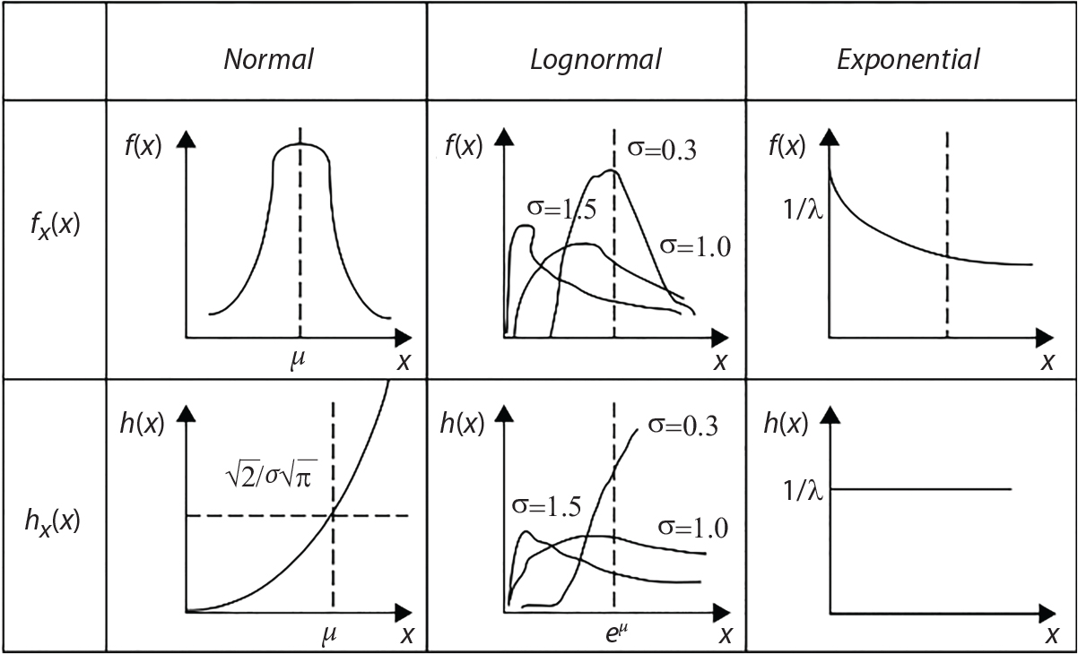
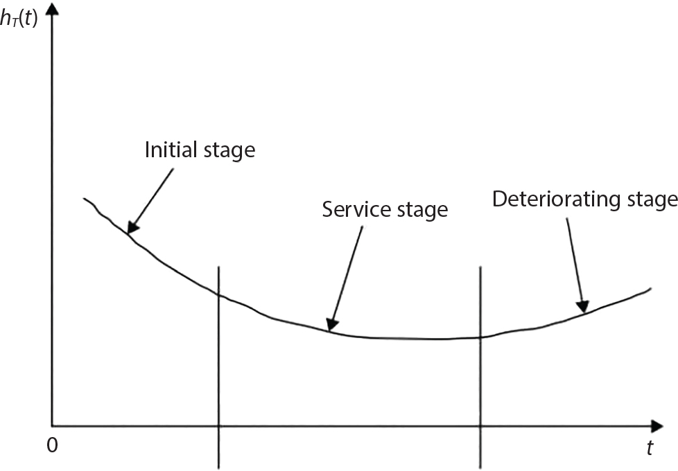
6.3 Calculation of Time-Dependent Reliability
6.3.1 Introduction

 will be replaced by the term
  .
.
6.3.2 Sampling Methods for Unconditional Failure Probability
 . Using conditional probability, the multiple integral can be written as:
 ; X1 and X2 in Equation (6.39) are subsets of random vector X;
  is the conditional PDF of X2 given X1; D1 and D2 are sample spaces of X1 and X2, respectively. D1 and D2 must be mutually exclusive and belong to D.
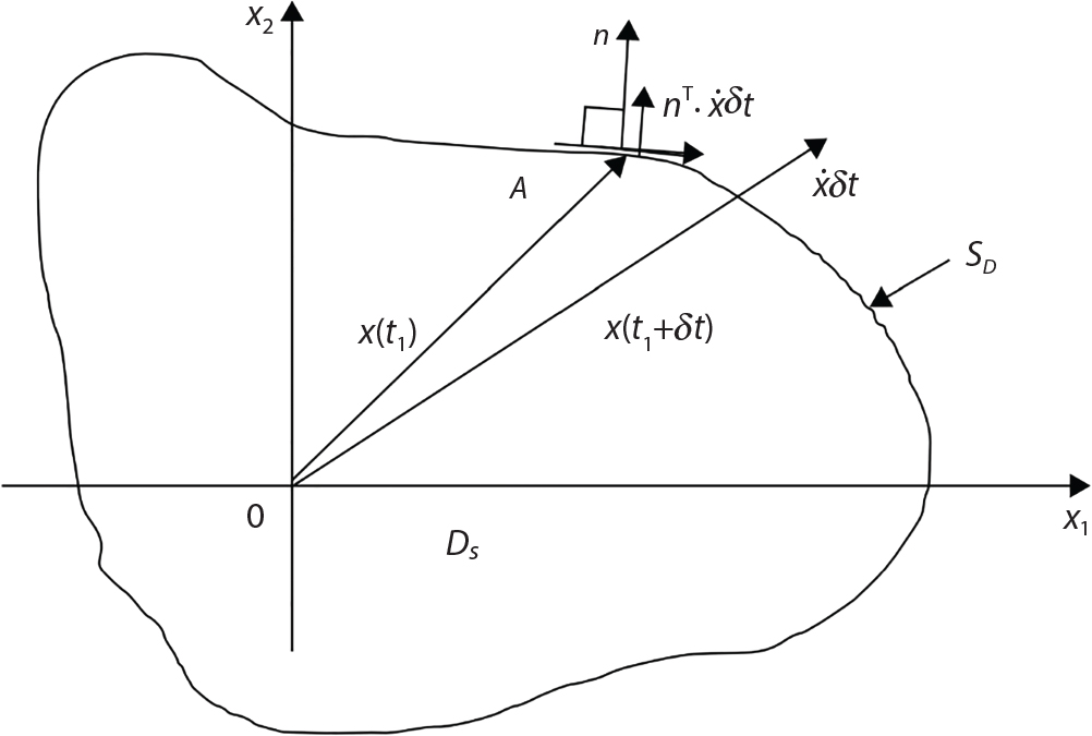
 and initial failure probability pf(0):
 represents the crossing rate at which vector random processes Q(t) leave the security domain D. Equation (6.42) can be adopted for directional simulation in vector random processes:
6.3.3 First-Order Second-Moment Method
 can be obtained by the first-order second-moment method. For every independent limit state equation, the conditional failure probability can be calculated using the upper boundary formula for crossing rate presented in Equation (6.41). If the load random process is a completely normal vector random process, the upper boundary of the first transcendence probability can be calculated by the first-order second-moment method with respect to Equation (6.38).
6.4 Structural Dynamic Analysis
6.4.1 Randomness of Structural Dynamics
6.4.2 Some Problems Involving Stationary Random Processes
 . Let uX = 0, and substitute it into Equation (6.44) and Equation (6.45), obtaining Equation (6.46):
 .
.  is the probability of transcendence offered in Equation (6.47);
  is the probability of transcending X = 0; when 0 ≤ a ≤ ∞, Equation (6.48) can be obtained:
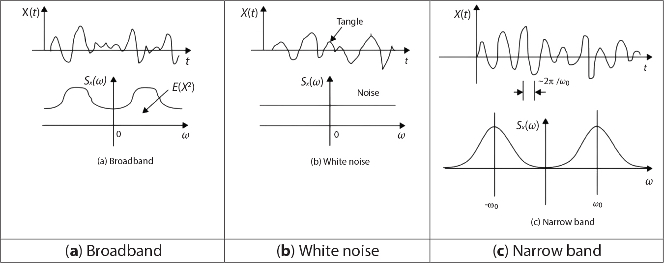
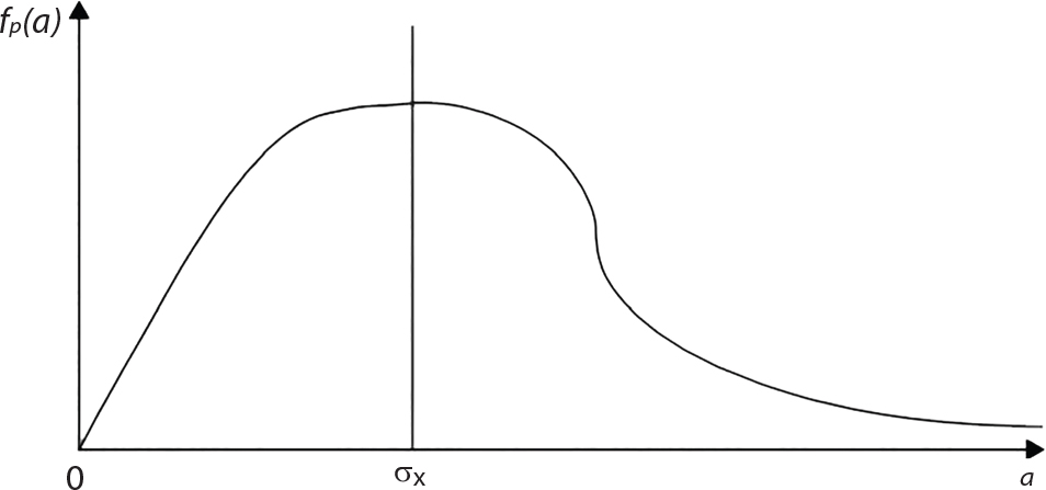
6.4.3 Random Response Spectrum
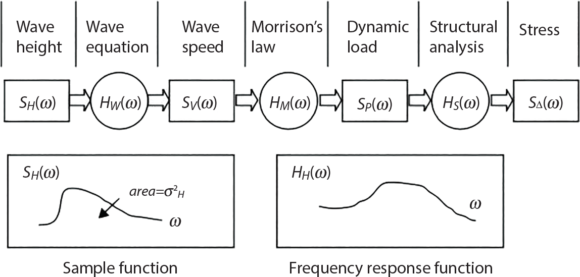
6.5 Fatigue Analysis
6.5.1 General Formulas
6.5.2 S-N Model
6.5.3 Fracture Mechanics Model
6.5.4 Example: Fatigue Reliability of an Offshore Jacket Platform
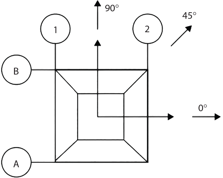
HS/m
p
TZ/S
Waves and current flow in the same direction
Waves and current are perpendicular to each other
FUS/kN
FZS/kN
FUS/kN
FZS/kN
0.25
0.15000
4.0
0.4
0.1
0.6
0.1
0.75
0.17500
4.0
5.5
1.3
7.4
1.6
1.25
0.11, 000
4.2
17.5
5.2
23.6
6.5
1.75
0.03750
4.7
37.4
13.1
50.6
16.3
2.25
0.01700
5.2
66.1
26.2
89.3
32.6
2.75
0.00600
5.6
104.0
45.5
146.0
56.6
3.25
0.00300
6.1
151.7
72.1
205.2
89.7
3.75
0.00100
6.6
209.7
106.8
283.5
133.0
4.25
0.00030
7.0
278.3
150.8
376.3
187.6
4.75
0.00015
7.4
357.8
208.0
483.9
254.8
5.25
0.00005
7.8
448.7
269.6
606.8
335.5
HS/m
p
TZ/S
Waves and current flow in the same direction
Waves and current are perpendicular to each other
FUS/kN
FZS/kN
FUS/kN
FZS/kN
0.25
0.15000
90.0
3.9
2.25
2.0
1.4
0.75
0.17500
90.0
43.1
15.4
26.5
9.0
1.25
0.11 000
90.0
131.3
37.4
80.4
22.0
1.75
0.03750
90.0
272.4
67.2
167.6
39.4
2.25
0.01700
90.0
470.4
104.2
289.1
61.0
2.75
0.00600
90.0
727.2
147.8
446.9
86.5
3.25
0.00300
90.0
1044.7
197.7
642.9
115.8
3.75
0.00100
90.0
1426.9
253.6
878.1
148.6
4.25
0.00030
90.0
1872.8
315.4
1152.5
184.6
4.75
0.00015
90.0
2384.3
382.8
1467.1
224.2
5.25
0.00005
90.0
2964.5
455.7
1823.8
267.0
Hd/m
Waves and current flow in the same direction
Waves and current perpendicular to each other
FUS/kN
FZS/kN
FUS/kN
FZS/kN
High frequency mooring force
0.25
10.74
6.29
14.16
7.83
1.00
52.35
31.45
70.79
39.14
1.75
115.17
69.20
155.75
86.11
2.50
177.98
106.94
240.70
133.08
3.25
240.80
144.69
325.65
180.05
4.00
303.62
182.43
410.60
227.02
4.75
366.44
220.17
495.55
273.99
5.50
429.26
257.92
580.51
320.96
6.25
492.07
295.66
665.46
367.93
7.00
554.89
333.41
750.41
414.90
7.75
617.71
371.15
835.36
461.90
8.50
680.53
408.89
920.31
508.84
9.25
743.35
446.64
1005.27
555.81
10.00
806.16
484.38
1090.22
602.78
10.75
868.98
522.13
1175.17
649.75
High frequency mooring force
0.25
70.58
10.85
43.42
6.36
1.00
352.92
54.25
217.12
31.78
1.75
776.42
119.35
477.66
69.72
2.50
1199.92
184.45
738.20
108.05
3.25
1 623.42
249.55
998.74
146.19
4.00
2 046. 92
314.65
1 259.28
184.32
4.75
2 470.42
379.75
1 519.28
222.46
5.50
2 893.92
444.85
1 780.36
260.60
6.25
3 317.42
509.95
2 040. 90
298.73
7.00
3 740.92
575.05
2 301.44
336.87
7.75
4164. 42
640.15
2 561.98
375.0
8.50
4587. 92
705.25
2822. 52
413. I4
9.25
5011. 42
770.35
3083. 06
451.28
10.00
5434. 92
835.45
3343. 60
489.41
10.75
5 858. 42
900.55
3604. 14
527.55
Hd/m
HS/m
0.25
0.75
1.25
1.75
2.25
2.75
3.25
3.75
4.25
4.75
5.25
0.25
340851
91641
21167
3354
838
185
61
14
3
1
0
1.00
53349
355122
177599
36867
10378
2433
831
197
44
17
4
1.75
0
13129
71085
32300
12901
3635
1383
351
82
33
9
2.50
0
0
5370
9935
7340
2854
1312
376
95
40
1
3.25
0
0
92
1331
2380
1467
883
300
86
39
12
4.00
0
0
0
0
468
526
450
191
63
32
10
4.75
0
0
0
0
57
135
178
99
40
23
8
5.50
0
0
0
0
4
25
55
43
1
14
6
6.25
0
0
0
0
0
3
4
5
10
8
4
7.00
0
0
0
0
0
0
3
5
4
4
2
7.75
0
0
0
0
0
0
0
1
1
2
1
8.50
0
0
0
0
0
0
0
0
0
1
1
9.25
0
0
0
0
0
0
0
0
0
0
0
10.00
0
0
0
0
0
0
0
0
0
0
0
10.75
0
0
0
0
0
0
0
0
0
0
0
Hd/m
HS/m
0.25
0.75
1.25
1.75
2.25
2.75
3.25
3.75
4.25
4.75
5.25
0.25
15 149
4073
988
175
48
12
4
1
0
0
0
1.00
2371
15 783
8288
1925
600
151
56
14
3
1
0
1.75
0
584
3317
1687
745
226
94
26
6
3
1
2.50
0
0
251
519
424
178
89
28
7
3
1
3.25
0
0
4
70
138
91
60
22
7
3
1
4.00
0
0
0
4
27
33
31
14
5
3
1
4.75
0
0
0
0
3
8
12
7
3
2
1
5.50
0
0
0
0
0
2
4
3
2
1
1
6.25
0
0
0
0
0
0
1
1
1
1
0
7.00
0
0
0
0
0
0
3
0
0
0
0
7.75
0
0
0
0
0
0
0
0
0
0
0
8.50
0
0
0
0
0
0
0
0
0
0
0
9.25
0
0
0
0
0
0
0
0
0
0
0
10.00
0
0
0
0
0
0
0
0
0
0
0
10.75
0
0
0
0
0
0
0
0
0
0
0
 the average wave zero-crossing rate,
  low-frequency mooring force zero-crossing rate,
  high-frequency mooring force zero-crossing rate.
Node
Bar
Type of structural components
FSC
D
Tf/a
Axial
In-plane bending moment
In-plane bending moment
36
36-32
CHD
4.524
1. 833
3.261
0.0207
48.3
36-35
BRC
4.555
2.011
2.895
0.0219
45.6
36-40
CHD
6.104
2.027
4.297
0.0159
62.7
36-39
BRC
6.420
2.087
4.145
0.0181
55.4
36-40
CHD
6.104
2.027
4.297
0.0159
62.9
36-37
BRC
6.420
2.087
4. 145
0.0180
55.5
36-32
CHD
4.524
1. 833
3.261
0.0207
48.4
36-33
BRC
4. 555
2.011
2.895
0.0219
45.7
37
37-41
CHD
6.104
2.027
4.297
0.0163
61.2
37-38
BRC
6. 420
2.087
4.145
0.0186
53.9
37-4 1
CHD
6.104
2.027
4.297
0.0163
61.2
37-36
BRC
6.420
2.087
4.145
0.0185
54.0
38
38-34
CHD
4.524
1.833
3.261
0.0206
48.6
38-35
BRC
4.555
2.011
2.895
0.0218
45.9
38-42
CHD
6.104
2.027
4.297
0.0155
64.4
38-39
BRC
6.420
2.087
4.145
0.0176
56.8
38-42
CHD
6.104
2.027
4.297
0.0156
64.2
38-37
BRC
6.420
2.087
4.145
0.0176
56.7
38-34
CHD
4. 524
1.833
3.261
0.0206
48.5
38-33
BRC
4. 555
2.011
2.895
0.0219
45.7
39
39-43
CHD
6.104
2.027
4.297
0.0165
60.4
39-36
BRC
6.420
2.087
4.145
0.0188
53.2
39-43
CHD
6.104
2.027
4.297
0.0163
61.3
39-38
BRC
6.420
2.087
4.145
0.0185
54.0
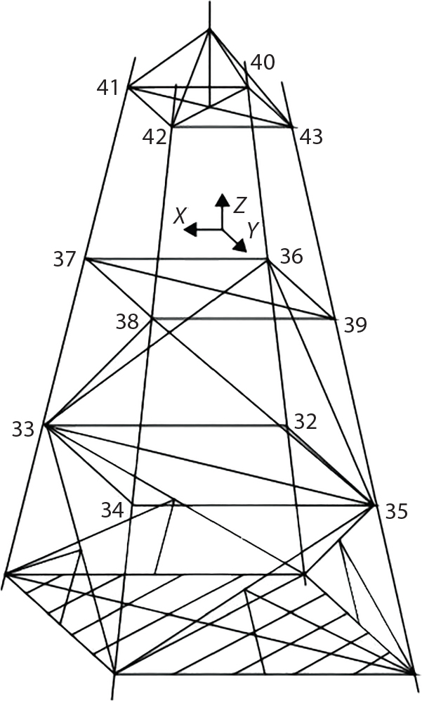
6.5.5 Example: Fatigue Reliability of a Submarine Pipeline and Analysis of its Parameters
6.5.5.1 Introduction
6.5.5.2 Analytical Process
6.5.5.3 Finite Element Model
6.5.5.4 Random Lift Model
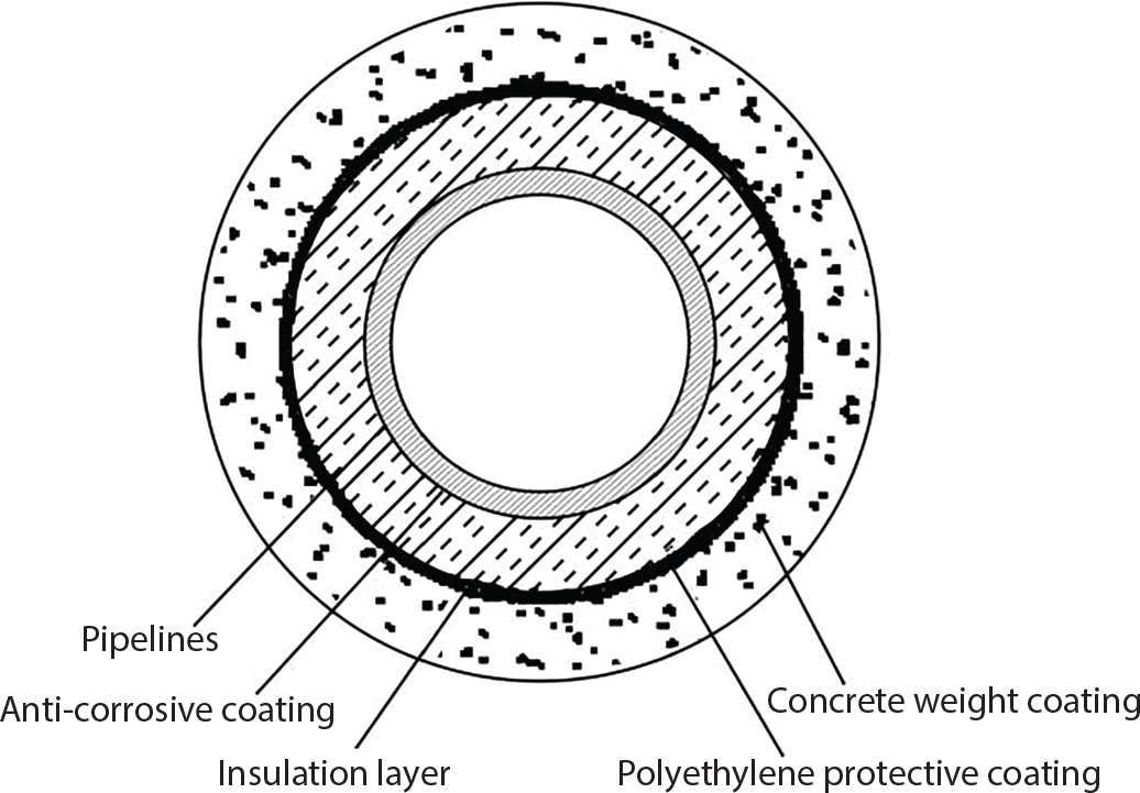
Materials
Size
Remarks
Pipeline
Steel (API 5L X65 SML)
Diameter 168.3mm wall 11.0mm thick
E=2.07×10⁵MPa
Anti-corrosive coating
Epoxy powder
0.4mm thick
Density 940kg/m3
Insulation layer
Polyurethane foam
40mm thick
Density 60kg/m3
Protective layer
Polyethylene
8mm thick
Waterproof
Weight coating
Concrete
40mm thick
Density 2950kg/m3
 ; ρ is the density of seawater; D is the outer diameter of the pipeline; u(t) is the horizontal velocity of the wave water quality point at the depth of the pipeline axis; CL is the lift coefficient.
 is the circular frequency of the waves; η(t) is the wave height function.
 is the transfer function for the horizontal velocity of the wave water point; Sη(ω) is the spectral wave density function.
 and the autocorrelation function of water particle velocity Ru(τ) can be expressed as:
6.5.5.5 Structural Modal Analysis
Mode
Case 1
Case 2
Case 3
Frequency (Hz)
Modal contribution rate
Frequency (Hz)
Frequency (Hz)
1
0.400
0.8379
0.625
1.111
2
1.102
0.1107
1.722
3.059
3
2.160
0.0289
3.373
5.989
4
3.568
0.0106
5.571
9.886
5
5.327
0.0048
8.314
14.742
6
7.435
0.0025
11.598
20.548
7
9.890
0.0014
15.421
27.294
8
12.691
0.0009
19.799
34.967
9
15.836
0.0006
24.666
43.555
10
19.323
0.0004
30.078
53.041
6.5.5.6 Random Vibration Response of Suspended Pipelines
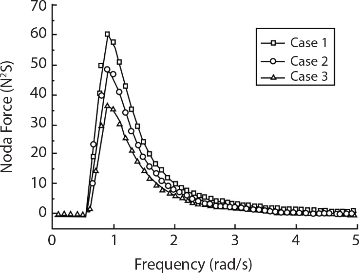
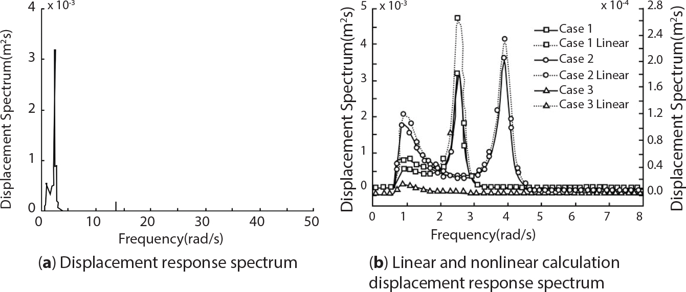
 , and N is the displacement interpolation function matrix, [N1,N2].
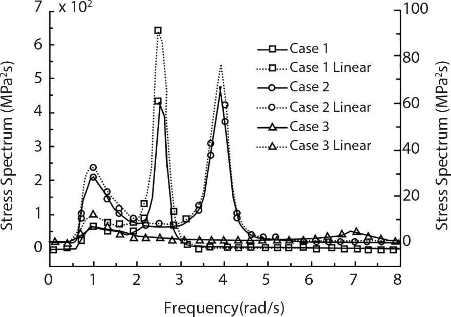
6.5.5.7 Random Fatigue Life and Fatigue Reliability Analysis of a Suspended Pipeline
Cases
Span length (m)
Annual cumulative damage
Fatigue life (y)
Reliability index
Failure probability
1
50.00
0.239
4.18
2.87
0.207×10⁻²
2
40.00
0.200×10⁻¹
0.50×10²
3.58
0.173×10⁻³
3
30.00
0.843×10⁻³
0.12×10⁴
4.34
0.730×10⁻⁵
1-Linear
50.00
0.692
1.45
2.51
0.599×10⁻²
2-Linear
40.00
0.342×10⁻¹
0.29×10²
3.43
0.296×10⁻³
3-Linear
30.00
0.942×10⁻³
0.11×10⁴
4.20
0.815×10⁻⁵
6.5.5.8 Sensitivity Analysis of Random Vibration Influencing Factors of a Suspended Pipeline
Span length (m)
Annual cumulative damage
Fatigue life (y)
Reliability index
Failure probability
30.00
0.843×10⁻³
0.12×10⁴
4.34
0.730×10⁻⁵
35.00
0.427×10⁻²
0.23×10²
3.96
0.370×10⁻⁴
40.00
0.200×10⁻¹
0.50×10²
3.58
0.173×10⁻³
45.00
0.567×10⁻¹
0.18×10²
3.30
0.491×10⁻³
50.00
0.239
4.18
2.87
0.207×10⁻²
Wave height (m)
Annual cumulative damage
Fatigue life (y)
Reliability index
Failure probability
2
0.122×10⁻¹
0.82×10²
3.71
0.105×10⁻³
3
0.200×10⁻¹
0.50×10²
3.58
0.173×10⁻³
4
0.430×10⁻¹
0.23×10²
3.37
0.372×10⁻³
5
0.823×10⁻¹
0.12×10²
3.19
0.712×10⁻³
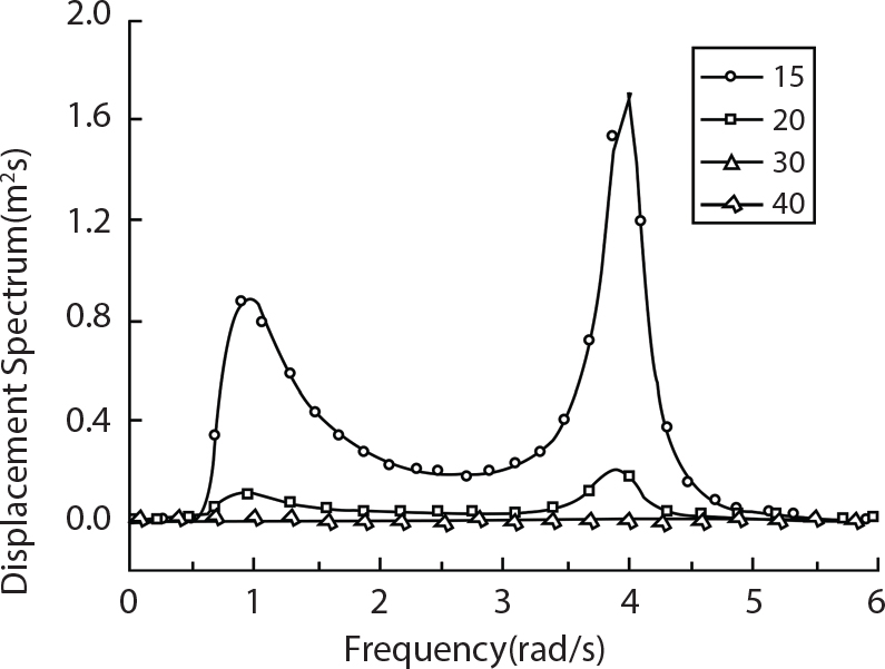
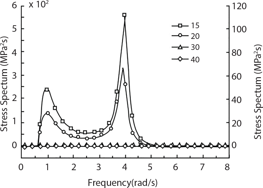

Pipeline depth (m)
Annual cumulative damage
Fatigue life (y)
Reliability index
Failure probability
15
0.200×101
0.50
2.11
0.174×10⁻¹
20
0.200×10⁻¹
0.50×10²
3.58
0.173×10⁻³
30
0.252×10⁻⁵
0.40×10⁶
5.48
0.218×10⁻⁷
40
0.251×10⁻⁹
0.40×10¹⁰
6.93
0.217×10⁻¹¹
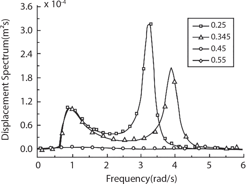
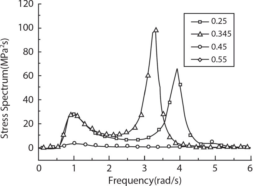
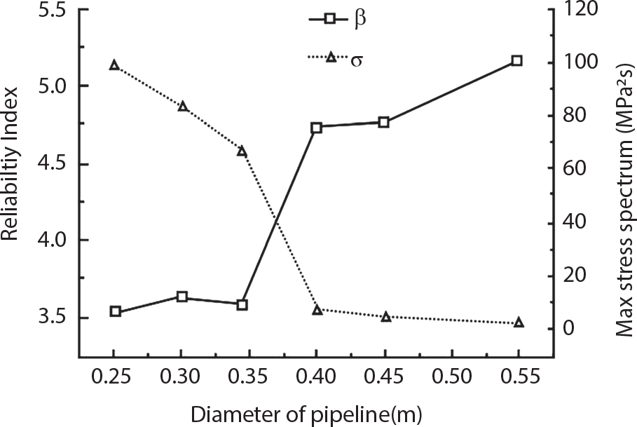
Pipeline diameter (m)
Annual cumulative damage
Fatigue life (y)
Reliability index
Failure probability
0.25
0.241×10⁻¹
0.41×10²
3.53
0.209×10⁻³
0.30
0.168×10⁻¹
0.60×10²
3.62
0.145×10⁻³
0.345
0.200×10⁻¹
0.50×10²
3.58
0.173×10⁻³
0.40
0.125×10⁻³
0.80×10⁴
4.74
0.108×10⁻⁵
0.45
0.112×10⁻³
0.89×10⁴
4.76
0.971×10⁻⁶
0.55
0.142×10⁻⁴
0.70×10⁵
5.16
0.123×10⁻⁶
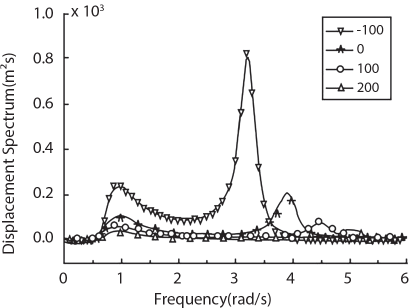
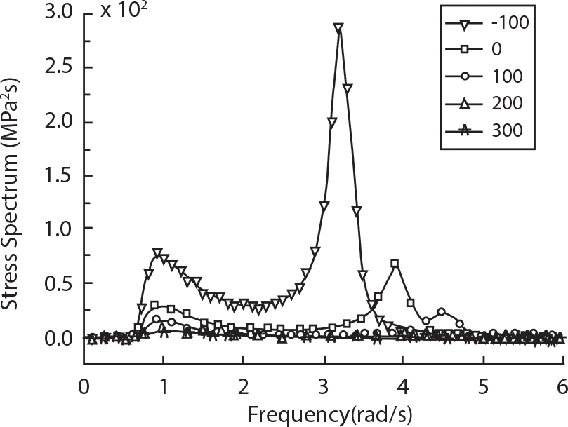
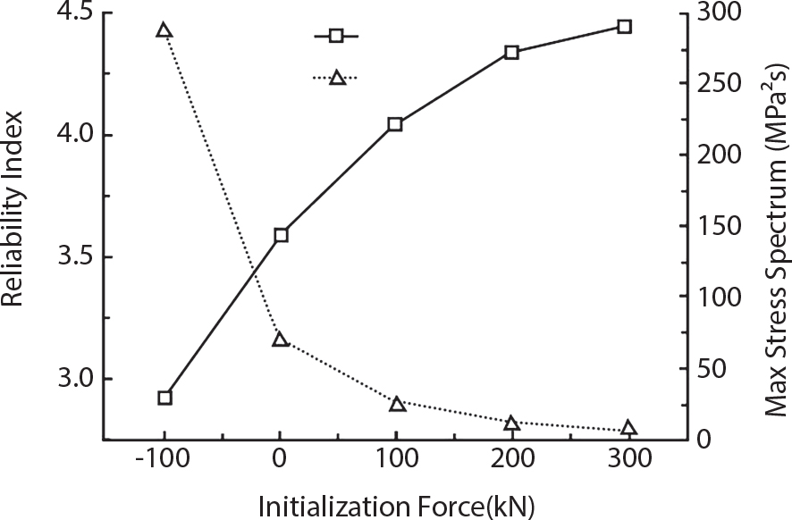
Axial force (kN)
Annual cumulative damage
Fatigue life (y)
Reliability index
Failure probability
-100
0.219
0.46×101
2.90
0.189×10⁻²
0
0.200×10⁻¹
0.50×10²
3.58
0.173×10⁻³
100
0.315×10⁻²
0.32×10³
4.04
0.273×10⁻⁴
200
0.812×10⁻³
0.12×10⁴
4.34
0.703×10⁻⁵
300
0.247×10⁻³
0.40×10⁴
4.44
0.443×10⁻⁵
6.5.6 Example: Fatigue Reliability of Deep-Water Semi-Submersible Platform Structures
6.5.6.1 Analytical Process for Fatigue Reliability
6.5.6.2 Fatigue Reliability Analysis of Key Platform Joints
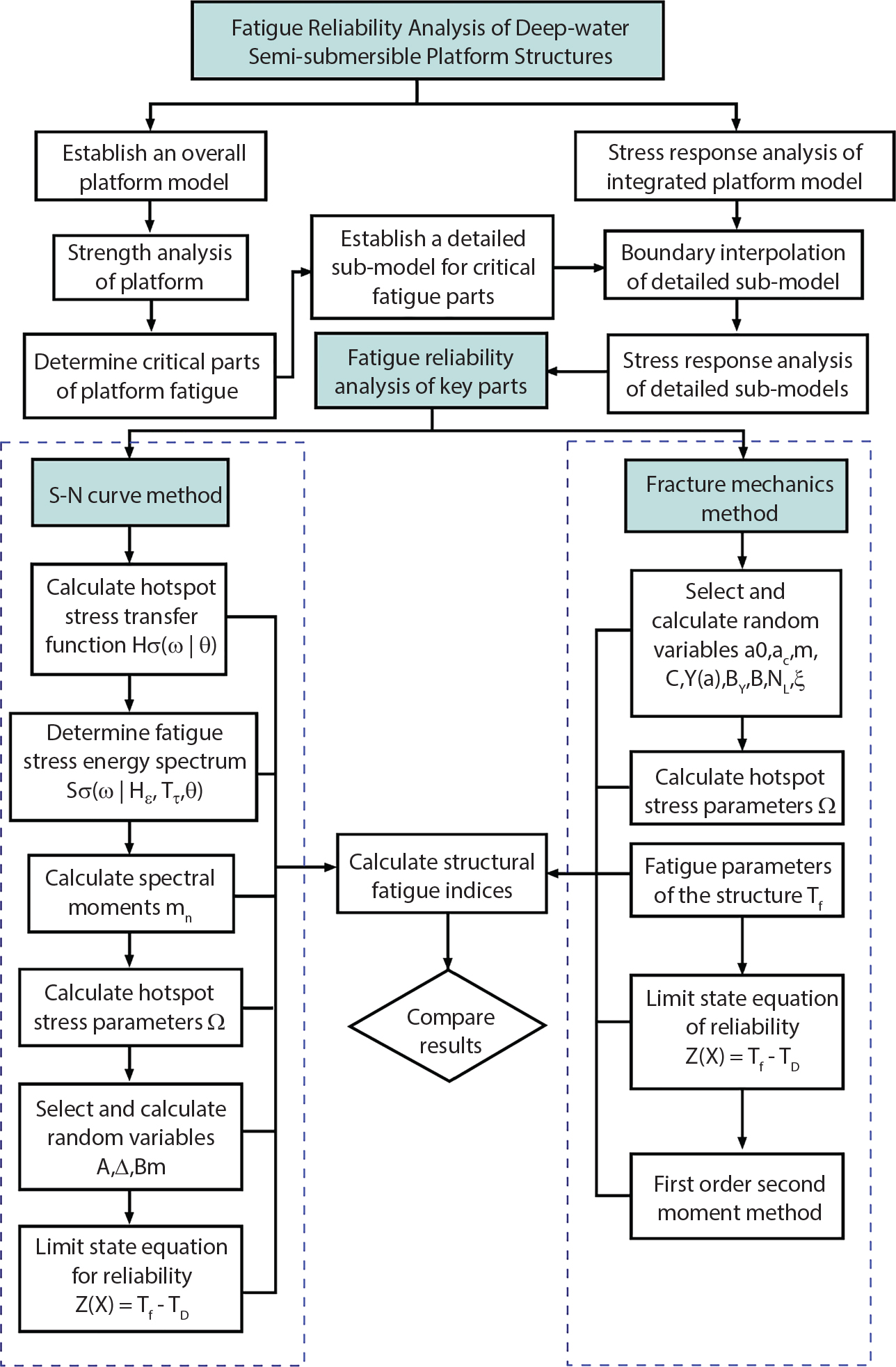
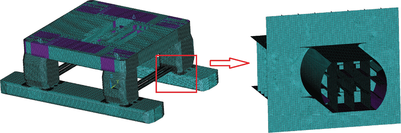
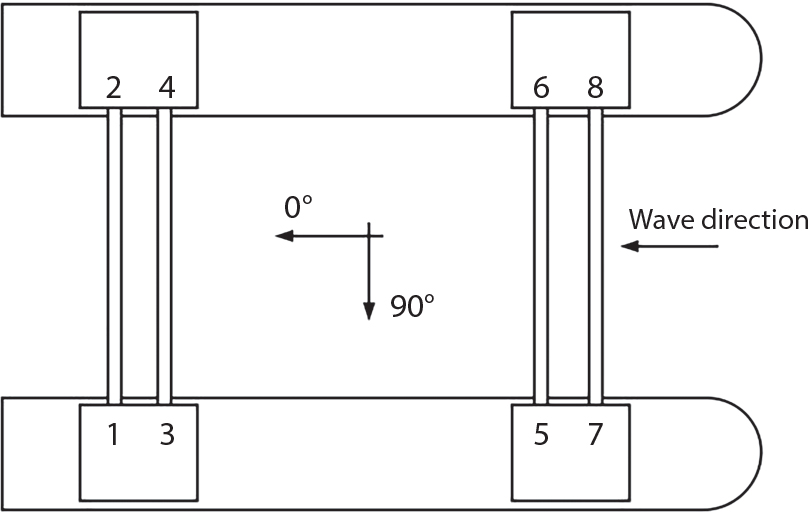
HS (m)
TZ (s)
<=3
3∼4
4∼5
5∼6
6∼7
7∼8
8∼9
9∼10
>10
0∼0.5
0.29
1.13
5.35
8.20
1.47
0.12
0.01
0.00
0.00
0.5∼1.0
0.05
0.67
7.05
6.61
4.62
1.64
0.30
0.03
0.00
1.0∼1.5
0.00
0.02
1.46
8.34
5.05
2.06
0.97
0.37
0.03
1.5∼2.0
0.00
0.00
0.00
2.24
7.91
2.21
1.09
0.69
0.16
2.0∼2.5
0.00
0.00
0.00
0.01
3.72
4.68
0.86
0.56
0.33
2.5∼3.0
0.00
0.00
0.00
0.00
0.13
4.29
1.67
0.34
0.34
3.0∼3.5
0.00
0.00
0.00
0.00
0.00
0.91
3.17
0.38
0.20
3.5∼4.0
0.00
0.00
0.00
0.00
0.00
0.05
1.81
1.00
0.23
4.0∼4.5
0.00
0.00
0.00
0.00
0.00
0.00
0.33
1.38
0.30
4.5∼5.0
0.00
0.00
0.00
0.00
0.00
0.00
0.03
0.81
0.46
5.0∼6.0
0.00
0.00
0.00
0.00
0.00
0.00
0.00
0.17
0.84
>6.0
0.00
0.00
0.00
0.00
0.00
0.00
0.00
0.02
0.86
Random variables
Values
Coefficient of variation
Fatigue strength coefficient, A
4.16×10¹¹
0.4
Structural fatigue damage degree, Δ
1.0
0.25
Uncertainty random variable in stress calculation, B
1.0
0.25
Fatigue index, m
3.0
–
Random variables
Values
Coefficient of variation
Initial crack size, a0 (mm)
0.5
1.00
Critical crack size, ac (mm)
25
–
Paris coefficient, C
2.3×10⁻¹²
0.25
Random uncertainty variable in stress calculation, B
1.0
0.25
Random uncertainty variables in the calculation of the geometric correction coefficient, BY
1.0
0.15
Paris coefficient, m
3.0
0.09
Threshold of fatigue crack growth, ΔKth (MPa·m1/2)
2
–
 ; R2 = t1−m/2, then
 , then the limit state function can be transformed into
 . The calculation above was carried out via computer programming in order to calculate the fatigue reliability index of the key fatigue node.
Connection part no.
Reliability index and failure probability
S-N curve method
A
B
C
D
1
β
6.840
5.997
5.736
4.825
Pf
3.960×10⁻¹²
1.005×10⁻⁹
4.847×10⁻⁹
7.000×10⁻⁷
2
β
7.354
6.565
5.625
4.689
Pf
9.618×10⁻¹⁴
2.602×10⁻¹¹
9.275×10⁻⁹
1.373×10⁻⁶
3
β
6.423
3.976
5.318
5.219
Pf
6.681×10⁻¹¹
3.504×10⁻⁵
5.246×10⁻⁸
8.995×10⁻⁸
4
β
5.453
3.496
5.075
5.812
Pf
2.476×10⁻⁸
2.361×10⁻⁴
1.937×10⁻⁷
3.087×10⁻⁹
5
β
5.644
3.018
5.244
5.485
Pf
8.307×10⁻⁹
1.272×10⁻³
7.857×10⁻⁸
2.067×10⁻⁸
6
β
6.158
4.139
5.196
5.421
Pf
3.683×10⁻¹⁰
1.744×10⁻⁵
1.018×10⁻⁷
2.963×10⁻⁸
7
β
5.549
5.415
4.891
3.924
Pf
1.437×10⁻⁸
3.064×10⁻⁸
5.016×10⁻⁷
4.355×10⁻⁵
8
β
5.830
5.096
5.631
5.358
Pf
2.771×10⁻⁹
1.735×10⁻⁷
8.958×10⁻⁹
4.207×10⁻⁸
6.5.6.3 Sensitivity Analysis of Fatigue Parameters
Connection part no.
Reliability index and failure probability
Fracture mechanics method
A
B
C
D
1
β
4.973
4.625
4.305
3.004
Pf
3.304×10⁻⁷
1.874×10⁻⁶
8.351×10⁻⁶
1.332×10⁻³
2
β
5.553
4.962
4.376
3.396
Pf
1.401×10⁻⁸
3.482×10⁻⁷
6.056×10⁻⁶
3.415×10⁻⁴
3
β
4.666
3.372
4.313
3.849
Pf
1.539×10⁻⁶
3.728×10⁻⁴
8.038×10⁻⁶
5.928×10⁻⁵
4
β
4.581
3.389
3.728
3.985
Pf
2.312×10⁻⁶
3.503×10⁻⁴
9.633×10⁻⁵
3.380×10⁻⁵
5
β
4.402
2.977
4.517
4.003
Pf
5.351×10⁻⁶
1.457×10⁻³
3.130×10⁻⁶
3.123×10⁻⁵
6
β
5.510
3.439
4.263
4.320
Pf
1.793×10⁻⁸
2.915×10⁻⁴
1.010×10⁻⁵
7.786×10⁻⁶
7
β
4.506
4.357
3.919
3.482
Pf
3.302×10⁻⁶
6.588×10⁻⁶
4.437×10⁻⁵
2.492×10⁻⁴
8
β
4.661
3.782
4.882
3.991
Pf
1.571×10⁻⁶
7.786×10⁻⁵
5.261×10⁻⁷
3.284×10⁻⁵
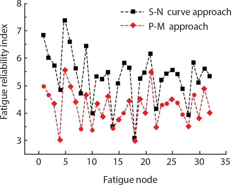
Curve type
In air
Curve type
Cathodic protection in seawater
Curve type
Free corrosion in seawater
A
m
A
m
A
m
B
1.01×10¹⁵
4
B
4.04×10¹⁴
4
B
3.37×10¹⁴
4
C
4.23×10¹³
3.5
C
1.69×10¹³
3.5
C
1.41×10¹³
3.5
D
1.52×10¹²
3
D
6.08×10¹¹
3
D
5.07×10¹¹
3
E
1.04×10¹²
3
E
4.16×10¹¹
3
E
3.47×10¹¹
3
F
6.30×10¹¹
3
F
2.52×10¹¹
3
F
2.10×10¹¹
3
G
2.50×10¹¹
3
G
1.00×10¹¹
3
G
8.33×10¹⁰
3
W
1.60×10¹¹
3
W
6.40×10¹⁰
3
W
5.33×10¹⁰
3
Curve type
In air
Cathodic protection in seawater
Free corrosion in seawater
1
2
3
4
1
2
3
4
1
2
3
4
B
8.87
7.94
7.53
6.34
8.87
7.94
7.53
6.34
8.71
7.77
7.36
6.17
C
8.29
7.40
7.06
5.98
8.29
7.40
7.06
5.98
8.10
7.21
6.87
5.80
D
7.28
6.43
6.17
5.26
7.28
6.43
6.17
5.26
7.07
6.23
5.96
5.05
E
6.84
6.00
5.74
4.83
6.84
6.00
5.74
4.83
6.63
5.79
5.53
4.62
F
6.26
5.42
5.16
4.25
6.26
5.42
5.16
4.25
6.05
5.21
4.95
4.04
G
5.20
4.36
4.10
3.19
5.20
4.36
4.10
3.19
4.99
4.15
3.89
2.97
W
5.74
4.90
4.64
3.73
4.69
3.84
3.58
2.67
4.48
3.63
3.37
2.46
References