Fractal geometry is the study of irregular shapes. Nature is full of these irregular shapes from trees and leaves, through mountains and rocks, to weather patterns and clouds. However these irregular shapes display a self-similarity across multiple scales that can be identified and used to inform our understanding. Nature’s self-similarity has a randomness to it. As an example, oak trees branch like oak trees and maple trees branch like maple trees from first branches to twigs, but all the branchings are not identical. Mathematics calls this self-affinity. The study of nature’s self-affinity was first presented by Benoit Mandelbrot in The Fractal Geometry of Nature. On the first page of the first chapter Mandelbrot asks the question,
Why is geometry often described as cold and dry? One reason lies in its inability to describe the shape of a cloud, a mountain, a coastline, or a tree. Clouds are not spheres, mountains are not cones, and coastlines are not circles, and bark is not smooth, nor does lightning travel in a straight line.
(Mandelbrot 1983, 1)
The fractal dimension is a measure of the irregularity of a shape. A prime mathematical example of an irregular self-similar entity is the Koch curve (Figure 8.1). The Koch curve is constructed through an iterative process. First a line segment is divided into thirds. Then the middle third of the curve is taken out and replaced with a triangular blip with sides equal in length to the thirds of the original line; thus the line is now four segments long. This procedure is then repeated on each of the now four line segments. The iterative process goes on to infinity in mathematical concept. In real world drawing of the Koch curve there is a limit to the iterations due to line width used to draw the curve. The fractal dimension as defined by Mandelbrot can be calculated as:
where a is the number of pieces and s is the reduction factor.
4 = (1/(1/3))D
4 = 3D
log (4) = D log (3)
D = log (4)/log (3)
D = 1.26
The dimension of the Koch curve tells us that it is more than a one-dimensional line and less than a two-dimensional plane. Other fractal curves have different fractal dimensions. The Cantor set, where a line is divided into thirds and then the middle third is taken out, has a fractal dimension of (D = log (2)/log (3) = 0.63). The Cantor set after many iterations reduces to a cluster of clusters of points. The Minkowski curve divides the original line into fourths and then constructs a line with eight segments. The fractal dimension of the Minkowski curve is (D = log (8)/log (4) = 1.5). The Peano curve divides the line into thirds and then creates a curve with nine segments creating a curve with the dimension (D = log (9)/log (3) = 2.0); thus the Peano curve is a line that, when iterated to infinity, will fill the two dimensional plane. As a comparison, a straight line divided into three segments that maintains the three segments has a dimension of (D = log (3)/log (3) = 1) (Bovill 1996, 23–27).
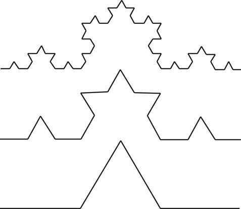
FIGURE 8.1 The Koch curve illustrates the construction of a fractal.
Source: Bovill 1996.
Mandelbrot asks the question, “How long is the coast of Britain?” (Mandelbrot 1983, 25). He comes to the conclusion that the length is undefinable because, as one uses a smaller and smaller measuring unit, the length gets longer and longer as more inlets and points are included in the measurement (Figure 8.2). However, a fractal dimension can be calculated for the coastline by measuring its length with shorter and shorter measuring units. Graphing the Log(coastline length) versus the log(1/length of the measuring unit) produces a straight line. The slope of the line is the measured dimension (d = 0.26). The fractal dimension is (D = 1 + d). Thus the fractal dimension of the coast of Britain is (D = 1.26). This is the same dimension as the Koch curve. Mandelbrot thus shows that nature is fractal (Bovill 1996, 27–38).
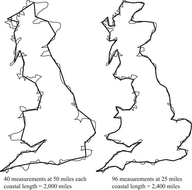
FIGURE 8.2 Measuring the length of the coast of England with smaller and smaller surveying distances produces longer and longer coastline lengths.
Source: Bovill 1996.
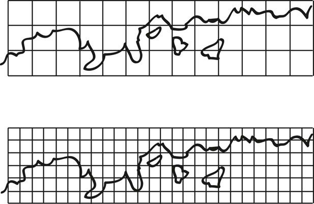
FIGURE 8.3 Measuring the fractal dimension of the coast line at Shell Beach, Sea Ranch, California with the box counting method.
Source: Bovill 1996.
Another slightly more flexible method of determining the fractal dimension of a shoreline is the box counting method. In this method a grid of boxes is drawn over the map of the coastline edge. Then a smaller grid of boxes is drawn over the same coastline. The number of boxes that the coastline runs through is counted in both cases. As an example, the fractal dimension of a short section of the coastline at the Sea Ranch in northern California can be determined by using a grid 400 feet square and a grid 200 feet square (Figure 8.3). At 400 feet there are 26 boxes with coastline in them. At 200 feet there are 65 boxes with coastline in them. The 400 foot box grid has 13 boxes across its long dimension. The 200 foot box grid has 26 boxes across its long dimension. The fractal dimension is determined by dividing the difference between the logs of the number of boxes across the long dimension of the box grids into the difference between the logs of the number of boxes with line in them. The fractal dimension of this coastline is equal to 1.32 (Bovill 1996, 41–42).
In constructing the Koch curve a line segment was divided into thirds, the middle third was erased, and a triangular blip was placed in the opening. Then this process was repeated for the four line segments to create blips on all four of them. This process is conceptually repeated to infinity. This is called iteration. A slightly different iterative process uses rectangular shapes that are reduced and mapped onto all of the original shapes. Four rectangles placed in the shape of a Koch curve, when iterated, creates the Koch curve. Michael Barnsley (1998) showed that the same four rectangles that could be used to produce a Koch curve, rearranged a different way, can create an iterated image of a life like fern with multiple self-similar leaves. The importance of Barnsley’s fern is that a natural looking fern can be produced with the same iterative procedures that produced the Koch curve and other fractal constructions. It also showed that complex natural forms can be produced with minimal starting information through iteration (Peitgen et al. 1992, 255–260).
Another form of iteration involves the use of simple equations in the complex plane. Complex numbers have a real number part and an imaginary number part. Imaginary numbers come from the fact that there is no solution to the square root of –1. No number multiplied by itself can result in –1. Mathematics solves this problem by using i to represent the square root of –1. Then i is used to indicate the imaginary part of a complex number z = x + yi. The complex plane is two dimensional. The horizontal axis is the real number scale, and the vertical axis is the imaginary number scale. Julia sets, named after Gaston Julia, are derived by iterating a simple equation z(n + 1) = z(n)2 + c, where c is a complex number. The iteration creates two sets. One set of results is unbounded so the numbers get very large. The other set is bounded. The Julia set is the boundary between these two sets of results. Julia sets are fractal in that structures repeat at different scales but not in an identical self-similar manner. They are self-affine; thus they are like natural fractals. Trees, coastlines, and mountain ridges display self-affine repetitions (Bovill 1996, 60–67).
Julia sets come in two varieties. Some Julia sets are all connected together, and some Julia sets are disconnected into a collection of separate components. Every Julia set has a complex number (x + yi) as its seed. Benoit Mandelbrot plotted on the complex plane the locations of the Julia sets that are and are not connected. The result is the Mandelbrot set (Figure 8.5). The colored-in area represents the area of the complex plane that produces connected Julia sets. The area outside the colored-in area is the area of the complex plane that produces disconnected Julia sets. The edge between these two areas is infinitely complex. Using a computer to zoom in on the edge of the Mandelbrot set at any point produces a never ending display of Julia set like forms, including small replicas of the Mandelbrot set (Bovill 1996, 68–70). YouTube has many videos zooming into the complex edges of the Mandelbrot Set. Search for “Mandelbrot set” or “Mandelbrot set zoom”. The infinitely complex boundary of the Mandelbrot set provides a good analogy for nature. Nature is infinitely complex, which gives it stability. Take a close look at the structure of trees (Figure 8.6). The upper branches are self-affine replicas of the whole tree. This cascade continues through about five levels of branching.
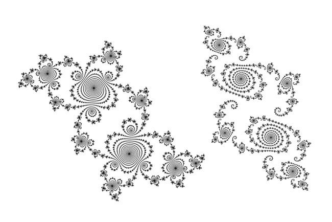
FIGURE 8.4 A connected Julia set and a disconnected Julia set.
Source: Wikimedia Commons, Attribution-Share Alike 3.0. Author Adam Majewski. Uploaded June 26, 2011. Wikipedia, Julia Set. http://en.wikipedia.org/wiki/Julia_Set.
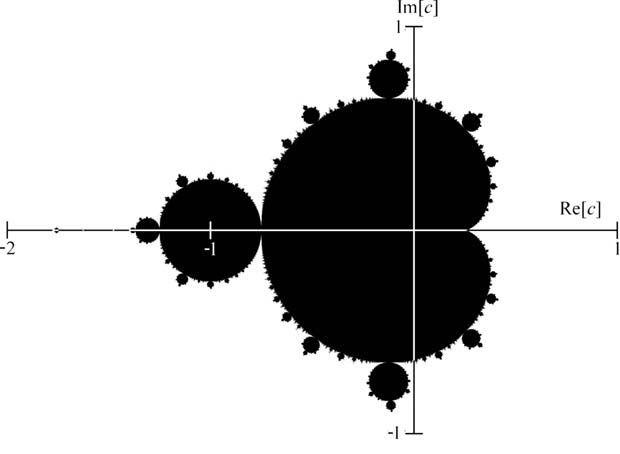
FIGURE 8.5 The Mandelbrot set is the intersection of the connected and disconnected Julia sets.
Source: Wikimedia Commons, Public Domain. Author Yourmomblah. Uploaded June 2, 2013. Wikipedia, Mandelbrot set. http://en.wikipedia.org/wiki/Mandelbrot_Set.
Edward Lorenz, experimenting with a set of three equations that represented a simplified model of the thermal functions that drive weather patterns in the atmosphere, inputted some rounded off numbers to start a computer run and discovered that the results were completely different from the original simulation. This is the chaos problem of sensitivity to initial conditions. Iterating the equations produces a strange attractor named the Lorenz attractor (Figure 8.7). The tiniest modification of the initial conditions produces wildly different solutions after a few iterations. The solutions loop around the attractor in very different ways after a few initial loops, even though the initial conditions were almost identical. This has a real world implication. Weather forecasting has limits. Even with improved data collection and improved computer simulations it is not possible to forecast the weather accurately beyond 5 to 10 days into the future. The atmosphere is a chaotic system (Peitgen et al. 1992, 697–708). If we cannot predict the weather even with a large number of accurate data points, how can we expect to manage the ecosystems of the earth?
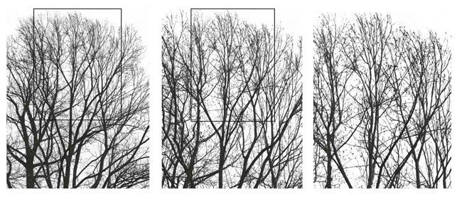
FIGURE 8.6 Zooming in on a stand of trees produces self-affine images.
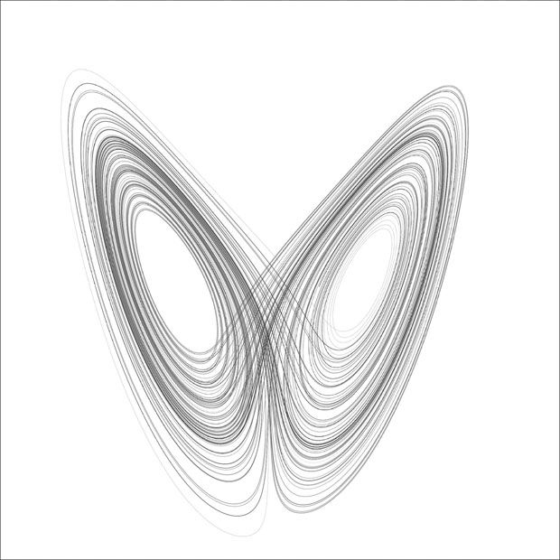
FIGURE 8.7 The Lorenz attractor.
Source: Wikimedia Commons, Attribution-Share Alike 3.0. Author Wikimol and Dshwin. Uploaded on January 4, 2006. Wikipedia, Chaos Theory. http://en.wikipedia.org/wiki/chaos_theory.
Another look into chaos can be seen by iterating the simple equation: (xn+1 = rxn(1 – xn). When this equation is iterated, with the parameter r set between 1 and 4, the results display the doubling route from stability to chaos. The Feigenbaum diagram, named after Michael Feigenbaum, shows how the solution to the equation bifurcates into two solutions, then four solutions, then eight solutions, and finally into a chaotic region where there are large numbers of solutions (Figure 8.8). But surprisingly there are windows of order in the chaotic region. Feigenbaum discovered that the ratio of the distances along the horizontal axis from one doubling point to the next doubling point is a constant across the whole diagram and is equal to 4.6692 …, referred to as the Feigenbaum constant. Years after the mathematical discovery of period doubling leading to chaos, experiments in fluid flows arrived at the same constant (Peitgen et al. 1992, 585–591).
Chaos theory demonstrates that there are limits to what is knowable. Natural systems are complex, and indeterminate. Human culture needs to accept this and tread lightly on nature. The bright side of chaos and its sensitive dependence on initial conditions is that small changes applied at the right time can create large modifications in future outcomes. This is sometimes called the butterfly effect (Gordon et al. 2006, 63).
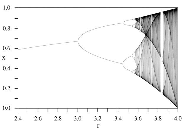
FIGURE 8.8 The Feigenbaum diagram shows the doubling cascade into chaos and the windows of order that can form in the chaotic region.
Source: Wikimedia Commons, Public Domain. Author PAR. Uploaded September 14, 2005. Wikipedia, Bifurcation Diagram. http://en.wikipedia.gov/wiki/Bifurcation_diagram.
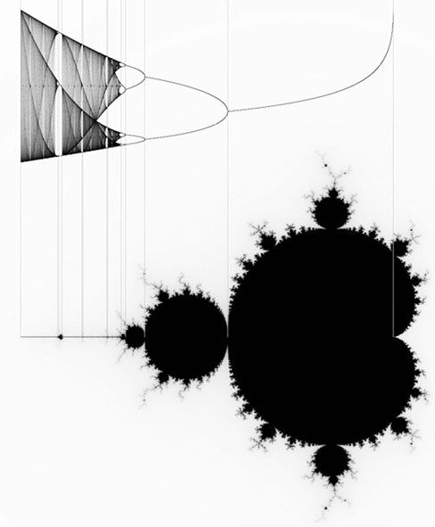
FIGURE 8.9 The relationship between the Feigenbaum diagram and the Mandelbrot set.
Source: Wikimedia, Public Domain, Author Georg-Johann Lay. Uploaded April 7, 2008. Wikipedia, Mandelbrot Set. http://en.wikipedia.org/wiki/Mandelbrot_Set.
In conclusion, a basic understanding of fractals and chaos can open up a new way of seeing the world (see Figure 8.10). Michael Barnsley, in the first chapter of his book Fractals Everywhere (1988), gives the following warning,
Fractal geometry will make you see everything differently. There is danger in reading further. You risk the loss of your childhood visions of clouds, forests, galaxies, leaves, flowers, rocks, mountains, torrents of water, carpets, bricks, and much else besides. Never again will your interpretation of these things be quite the same.
(Barnsley 1988, 1)
This statement applies equally to individuals and to human society as a whole.
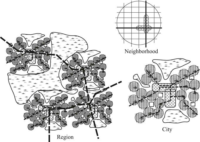
FIGURE 8.10 Urban environments show fractal characteristics. Walkable neighborhoods are connected into cities with local transportation systems, and the cities are connected into urban regions with regional transportation systems.